A confidence interval is a range of values that is likely to contain a population parameter with a certain level of confidence.
This tutorial explains how to plot a confidence interval for a dataset in R.
Example: Plotting a Confidence Interval in R
Suppose we have the following dataset in R with 100 rows and 2 columns:
#make this example reproducible
set.seed(0)

#create dataset
x #view first six rows of dataset
head(df)

           x          y
1  1.2629543  3.3077678
2 -0.3262334 -1.4292433
3  1.3297993  2.0436086
4  1.2724293  2.5914389
5  0.4146414 -0.3011029
6 -1.5399500 -2.5031813
To create a plot of the relationship between x and y, we can first fit a linear regression model:
model
Next, we can create a plot of the estimated linear regression line using the abline() function and the lines() function to create the actual confidence bands:
#get predicted y values using regression equation
newx #create plot of x vs. y, but don't display individual points (type='n')
plot(y ~ x, data = df, type = 'n')

#add fitted regression line
abline(model)

#add dashed lines for confidence bands
lines(newx, preds[ ,3], lty = 'dashed', col = 'blue')
lines(newx, preds[ ,2], lty = 'dashed', col = 'blue')
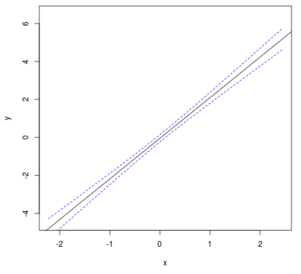
The black line displays the fitted linear regression line while the two dashed blue lines display the confidence intervals.
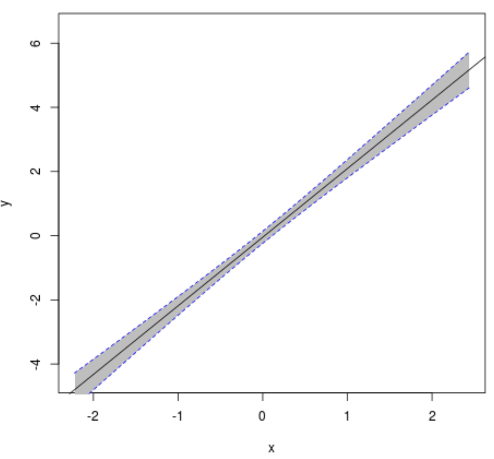
If you’d like, you can also fill in the area between the confidence interval lines and the estimated linear regression line using the following code:
#create plot of x vs. y
plot(y ~ x, data = df, type = 'n')

#fill in area between regression line and confidence interval
polygon(c(rev(newx), newx), c(rev(preds[ ,3]), preds[ ,2]), col = 'grey', border = NA)

#add fitted regression line
abline(model)

#add dashed lines for confidence bands
lines(newx, preds[ ,3], lty = 'dashed', col = 'blue')
lines(newx, preds[ ,2], lty = 'dashed', col = 'blue')
Here’s the complete code from start to finish:
#make this example reproducible
set.seed(0)

#create dataset
x
y
df

#fit linear regression model
model

#get predicted y values using regression equation
newx
preds

#create plot of x vs. y
plot(y ~ x, data = df, type = 'n')

#fill in area between regression line and confidence interval
polygon(c(rev(newx), newx), c(rev(preds[ ,3]), preds[ ,2]), col = 'grey', border = NA)

#add fitted regression line
abline(model)

#add dashed lines for confidence bands
lines(newx, preds[ ,3], lty = 'dashed', col = 'blue')
lines(newx, preds[ ,2], lty = 'dashed', col = 'blue')
Additional Resources
What are Confidence Intervals?
How to Use the abline() Function in R to Add Straight Lines to Plots