The following step-by-step example shows how to filter multiple columns in Google Sheets.
Step 1: Enter the Data
First, let’s enter the following data that shows the total sales of certain products in certain regions for a company:

Step 2: Apply Filter to Multiple Columns
Now suppose we’d like to filter for rows where the Region is “East” or the Product is “A.”
To do so, click cell A1 and then click the Data tab and then click Create a filter:

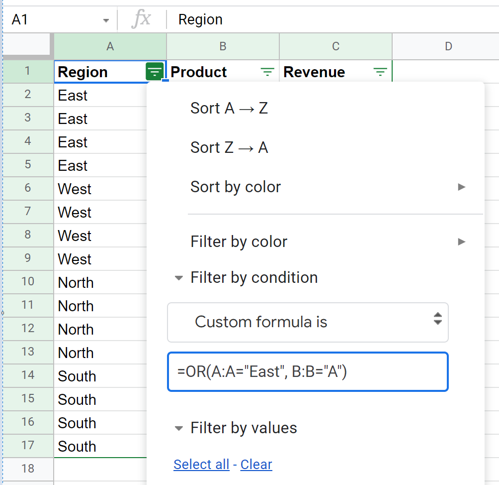
Next, click the Filter icon next to Region and then click Filter by condition.
In the dropdown menu, click None and then scroll down to Custom formula is and type in the following formula:
=OR(A:A="East", B:B="A")
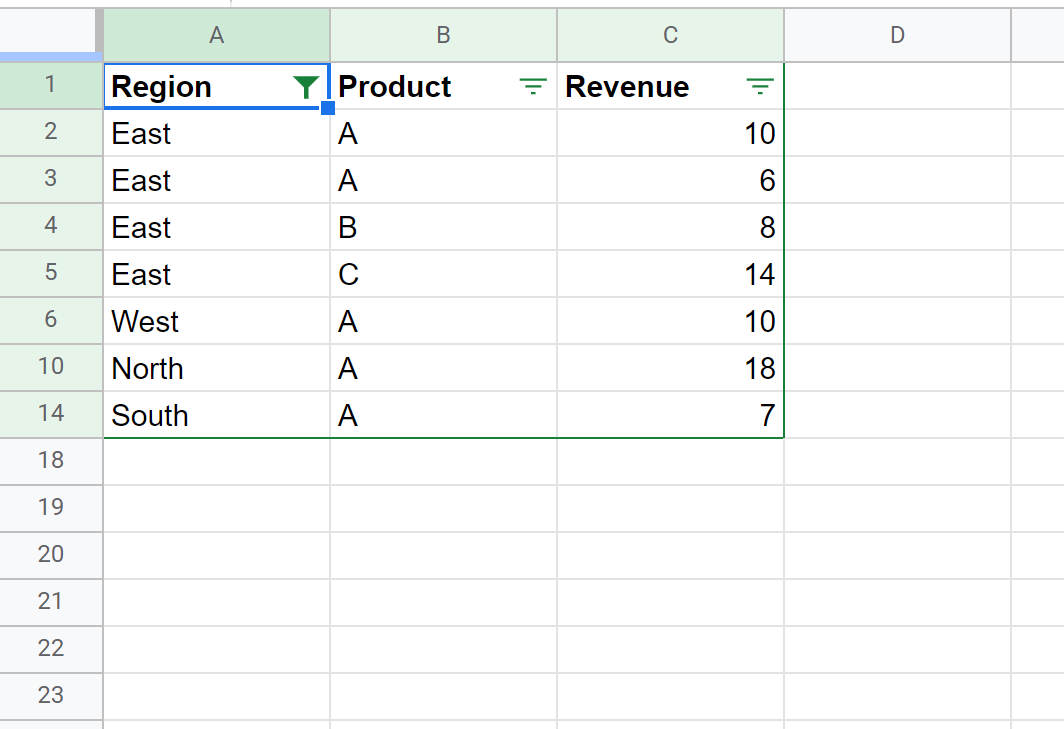
Once you click OK, the data will be filtered to only show rows where the Region is East or where the Product is A:
If you’d like to apply a filter where the Region is East and the Product is A, you can use the following formula:
=AND(A:A="East", B:B="A")
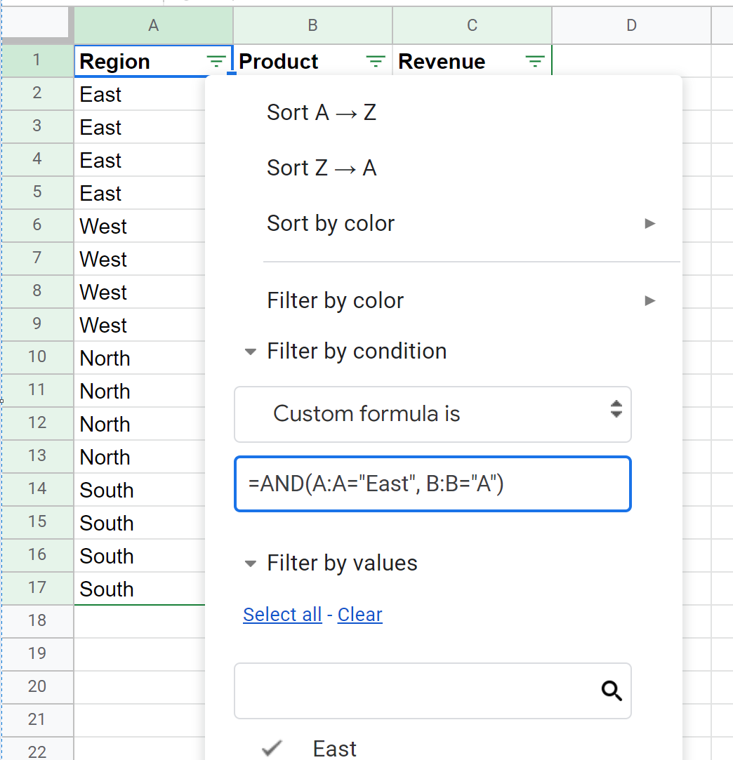
Once you click OK, the data will be filtered to only show rows where the Region is East and where the Product is A:

Additional Resources
The following tutorials explain how to perform other common operations in Google Sheets:
How to Sum Filtered Rows in Google Sheets
How to Use SUMIF with Multiple Columns in Google Sheets
How to Sum Across Multiple Sheets in Google Sheets