A histogram is a type of chart that allows us to visualize the distribution of values in a dataset.
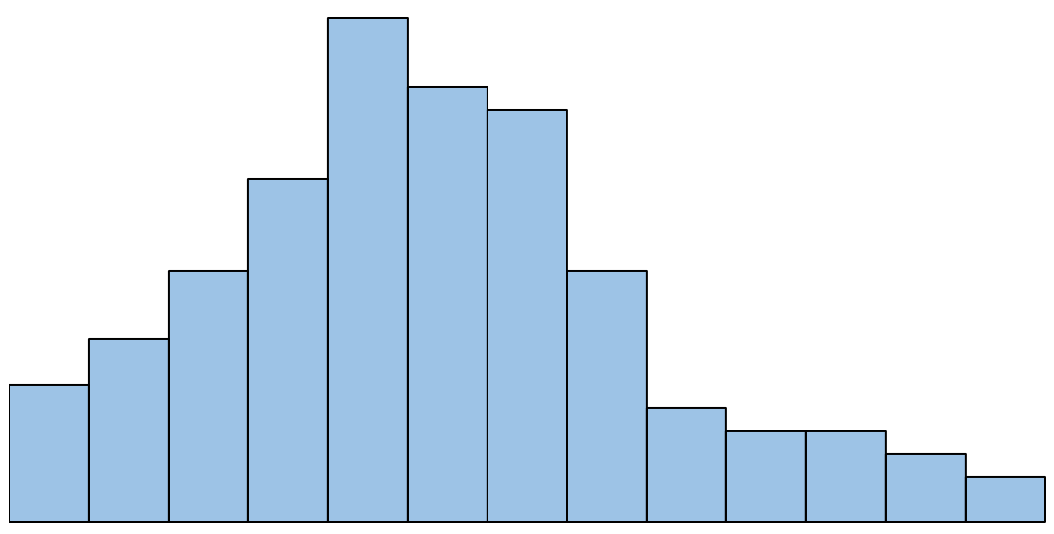
The x-axis displays the values in the dataset and the y-axis shows the frequency of each value.
Histograms are useful because they allow us to gain a quick understanding of the distribution of values in a dataset. They’re also useful for comparing two different datasets.
When comparing two or more histograms, we can answer three different questions:
1. How do the median values compare?
We can roughly estimate the median to be located near the middle of each histogram, which allows us to compare the median values of the distributions.
2. How does the dispersion compare?
We can visually see which histogram is more spread out, which gives us an idea of which distribution has values that are more dispersed.
3. How does the skewness compare?
If a histogram has a “tail” on the left side of the plot, it is said to be negatively skewed. Conversely, if a histogram has a “tail” on the right side of the plot, it is said to be positively skewed. We can visually check each histogram to compare the skewness.
The following example shows how to compare two different histograms and answer these three questions.
Example: Comparing Histograms
Suppose 200 students use one study method to prepare for an exam and another 200 students use a different study method to prepare for the same exam.
Suppose we create the following histograms to compare the exam scores for each group of students:

We can compare these histograms and answer the following three questions:
1. How do the median values compare?
Although we don’t know the exact median values of each distribution just by looking at the histograms, it’s obvious that the median exam score for students who used Method 1 is higher than the median exam score for students who used Method 2.
We might estimate that the median value for Method 1 is about 84 and the median value for Method 2 is about 78.
2. How does the dispersion compare?
The values in the histogram for Method 2 are much more spread out compared to the values for Method 1, which tells us that there is much greater dispersion in the exam scores for students who used Method 2.
3. How does the skewness compare?
From looking at the histograms, it appears that the distribution of exam scores for Method 1 is slightly right skewed, as indicated by the “tail” that extends to the right of the histogram.
There doesn’t appear to be any “tail” in the distribution of exam scores for Method 2, though, which tells us that the distribution has little to no skew.
Bonus: Here is the code that we used in R to create these two histograms:
library(ggplot2)

#make this example reproducible
set.seed(0)

#create data frame
df frame(method=rep(c('Method 1', 'Method 2'), each=200),
                 Score=c(rnorm(200, mean=84, sd=2),
                         rnorm(200, mean=78, sd=4)))

#create histogram of scores for each method
ggplot(df, aes(x=Score)) +
  geom_histogram(fill='steelblue', color='black') +
  facet_wrap(.~method, nrow=2) +
  labs(title='Exam Scores by Study Method')
Additional Resources
The following tutorials explain how to perform other common tasks with histograms:
How to Estimate the Mean and Median of Any Histogram
How to Estimate the Standard Deviation of Any Histogram
How to Describe the Shape of Histograms