Google Sheets Query: How to Join Two Tables

Often you may want to use the QUERY() function in Google Sheets to join two tables together.

Unfortunately, a JOIN() function does not exist within the QUERY() function, but you can use the following formula as a workaround to join two tables together:

=ArrayFormula(
   {
     A2:B6,
     vlookup(A2:A6,D2:E6,COLUMN(Indirect("R1C2:R1C"&COLUMNS(D2:E6),0)),0)
   }
)

This particular formula performs a left join on the tables located in the ranges A2:B6 and D2:E6.

The following example shows how to use this formula in practice.

Example: Join Two Tables in Google Sheets

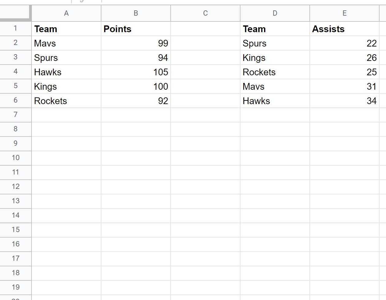
Suppose we have the following two tables in Google Sheets that contain information about various basketball teams:

We can use the following formula to perform a left join on the two tables and return one table that contains the team name, points, and assists for every team in the left table:

=ArrayFormula(
   {
     A2:B6,
     vlookup(A2:A6,D2:E6,COLUMN(Indirect("R1C2:R1C"&COLUMNS(D2:E6),0)),0)
   }
)

The following screenshot shows how to use this formula in practice:

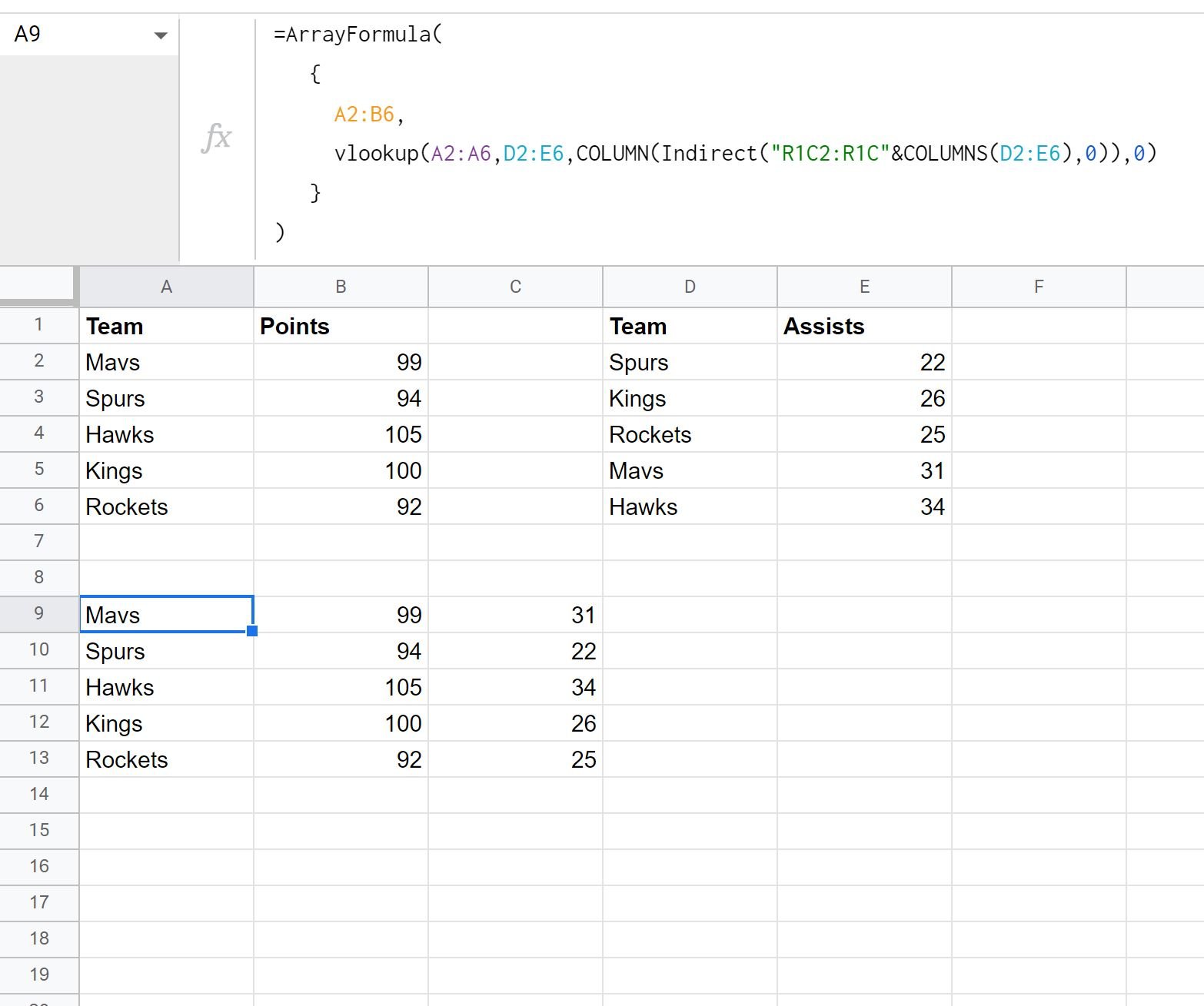
Notice that the result is one table that contains the team name, points, and assists for every team in the left table.

Note: If a team in the left table does not exist in the right table, a value of #N/A will be returned in the Assists column of the resulting table.

Additional Resources

The following tutorials explain how to perform other common tasks in Google Sheets

Google Sheets Query: How to Query From Another Sheet
Google Sheets Query: Select Rows that Contain String
Google Sheets Query: How to Use Group By