When the relationship between a set of predictor variables and a response variable is highly complex, we often use non-linear methods to model the relationship between them.
One such method is building a decision tree. However, the downside of using a single decision tree is that it tends to suffer from high variance. That is, if we split the dataset into two halves and apply the decision tree to both halves, the results could be quite different.
One method that we can use to reduce the variance of a single decision tree is to build a random forest model, which works as follows:
1. Take b bootstrapped samples from the original dataset.
2. Build a decision tree for each bootstrapped sample.
- When building the tree, each time a split is considered, only a random sample of m predictors is considered as split candidates from the full set of p predictors. Typically we choose m to be equal to √p.
3. Average the predictions of each tree to come up with a final model.
It turns out that random forests tend to produce much more accurate models compared to single decision trees and even bagged models.
This tutorial provides a step-by-step example of how to build a random forest model for a dataset in R.
Step 1: Load the Necessary Packages
First, we’ll load the necessary packages for this example. For this bare bones example, we only need one package:
library(randomForest)
Step 2: Fit the Random Forest Model
For this example, we’ll use a built-in R dataset called airquality which contains air quality measurements in New York on 153 individual days.
#view structure of airquality dataset
str(airquality)

'data.frame':	153 obs. of  6 variables:
 $ Ozone  : int  41 36 12 18 NA 28 23 19 8 NA ...
 $ Solar.R: int  190 118 149 313 NA NA 299 99 19 194 ...
 $ Wind   : num  7.4 8 12.6 11.5 14.3 14.9 8.6 13.8 20.1 8.6 ...
 $ Temp   : int  67 72 74 62 56 66 65 59 61 69 ...
 $ Month  : int  5 5 5 5 5 5 5 5 5 5 ...
 $ Day    : int  1 2 3 4 5 6 7 8 9 10 ...

#find number of rows with missing values
sum(!complete.cases(airquality))

[1] 42
This dataset has 42 rows with missing values, so before we fit a random forest model we’ll fill in the missing values in each column with the column medians:
#replace NAs with column medians
for(i in 1:ncol(airquality)) {
  airquality[ , i][is.na(airquality[ , i])] median(airquality[ , i], na.rm=TRUE)
}
Related: How to Impute Missing Values in R
The following code shows how to fit a random forest model in R using the randomForest() function from the randomForest package.
#make this example reproducible
set.seed(1)

#fit the random forest model
model #display fitted model
model

Call:
 randomForest(formula = Ozone ~ ., data = airquality)
               Type of random forest: regression
                     Number of trees: 500
No. of variables tried at each split: 1

          Mean of squared residuals: 327.0914
                    % Var explained: 61

#find number of trees that produce lowest test MSE
which.min(model$mse)

[1] 82

#find RMSE of best model
sqrt(model$mse[which.min(model$mse)])

[1] 17.64392
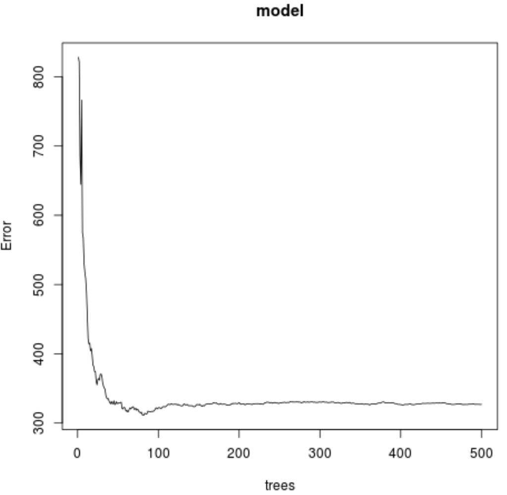
From the output we can see that the model that produced the lowest test mean squared error (MSE) used 82 trees.
We can also see that the root mean squared error of that model was 17.64392. We can think of this as the average difference between the predicted value for Ozone and the actual observed value.
We can also use the following code to produce a plot of the test MSE based on the number of trees used:
#plot the test MSE by number of trees
plot(model)

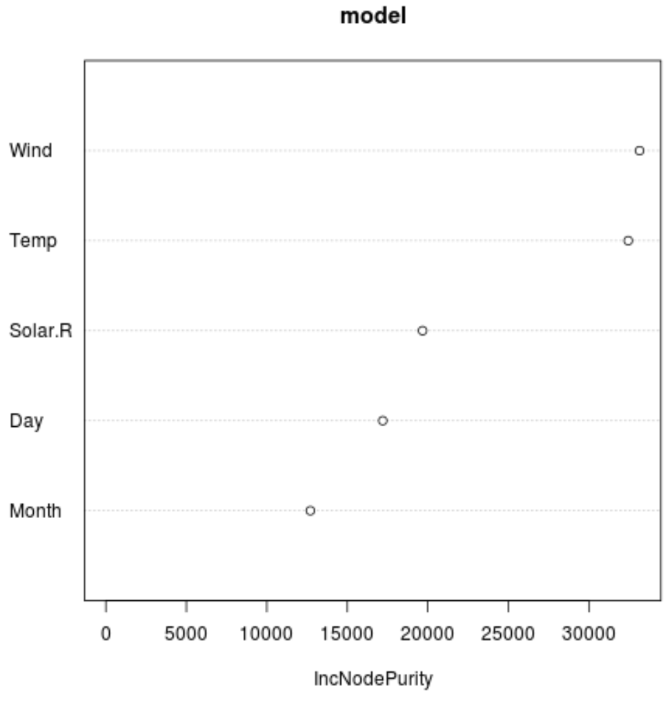
And we can use the varImpPlot() function to create a plot that displays the importance of each predictor variable in the final model:
#produce variable importance plot
varImpPlot(model)

The x-axis displays the average increase in node purity of the regression trees based on splitting on the various predictors displayed on the y-axis.
From the plot we can see that Wind is the most important predictor variable, followed closely by Temp.
Step 3: Tune the Model
By default, the randomForest() function uses 500 trees and (total predictors/3) randomly selected predictors as potential candidates at each split. We can adjust these parameters by using the tuneRF() function.
The following code shows how to find the optimal model by using the following specifications:
- ntreeTry: The number of trees to build.
- mtryStart: The starting number of predictor variables to consider at each split.
- stepFactor: The factor to increase by until the out-of-bag estimated error stops improving by a certain amount.
- improve: The amount that the out-of-bag error needs to improve by to keep increasing the step factor.
model_tuned #define predictor variables
               y=airquality$Ozone, #define response variable
               ntreeTry=500,
               mtryStart=4,
               stepFactor=1.5,
               improve=0.01,
               trace=FALSE #don't show real-time progress
               )
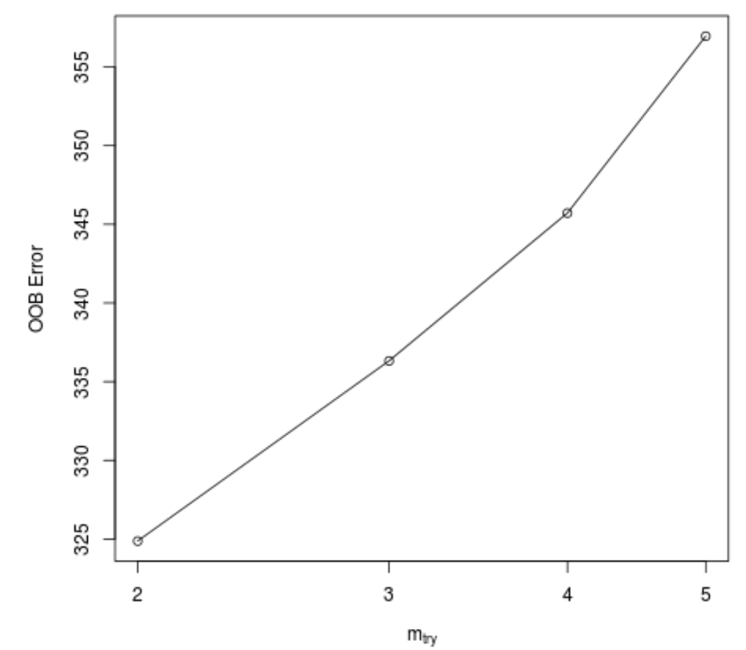
This function produces the following plot, which displays the number of predictors used at each split when building the trees on the x-axis and the out-of-bag estimated error on the y-axis:

We can see that the lowest OOB error is achieved by using 2 randomly chosen predictors at each split when building the trees.
This actually matches the default parameter (total predictors/3 = 6/3 = 2) used by the initial randomForest() function.
Step 4: Use the Final Model to Make Predictions
Lastly, we can use the fitted random forest model to make predictions on new observations.
#define new observation
new #use fitted bagged model to predict Ozone value of new observation
predict(model, newdata=new)

27.19442
Based on the values of the predictor variables, the fitted random forest model predicts that the Ozone value will be 27.19442 on this particular day.
The complete R code used in this example can be found here.