The Satterthwaite approximation is a formula used to find the “effective degrees of freedom” in a two-sample t-test.
It used most commonly in Welch’s t-test, which compares the means of two independent samples without assuming that the populations the samples came from have equal variances.
The formula for the Satterthwaite approximation is as follows:
Degrees of freedom: (s12/n1 + s22/n2)2 / {[(s12/n1)2/(n1 – 1)] + [(s22/n2)2/(n2 – 1)]}
where:
- s12, s22: The sample variance of the first and second sample, respectively.
- n1, n2: The sample size of the first and second sample, respectively.
The following example shows how to use the Satterthwaite approximation to calculate the effective degrees of freedom.
Example: Calculating the Satterthwaite approximation
Suppose we want to know if the mean height of two different plant species is equal so we go out and collect two simple random samples of each species and measure the height of the plants in each sample.
The following values show the height (in inches) for each sample:
Sample 1: 14, 15, 15, 15, 16, 18, 22, 23, 24, 25, 25
Sample 2: 10, 12, 14, 15, 18, 22, 24, 27, 31, 33, 34, 34, 34
The means, variances, and sample sizes turn out to be:
- x1 = 19.27
- x2 = 23.69
- s12 = 20.42
- s22 = 83.23
- n1 = 11
- n2 =13
Next, we can plug in the values for the variances and sample sizes into the Satterthwaite approximation formula to find the effective degrees of freedom:
df = (s12/n1 + s22/n2)2 / {[(s12/n1)2/(n1 – 1)] + [(s22/n2)2/(n2 – 1)]}

df = (20.42/11 + 83.23/13)2/{[(20.42/11)2/(11 – 1)] + [(83.23/13)2/(13 – 1)]} = 18.137
The effective degrees of freedom turns out to be 18.137.
Typically we round this value down to the next nearest integer, so the degrees of freedom that we would use in our Welch’s t-test is 18.
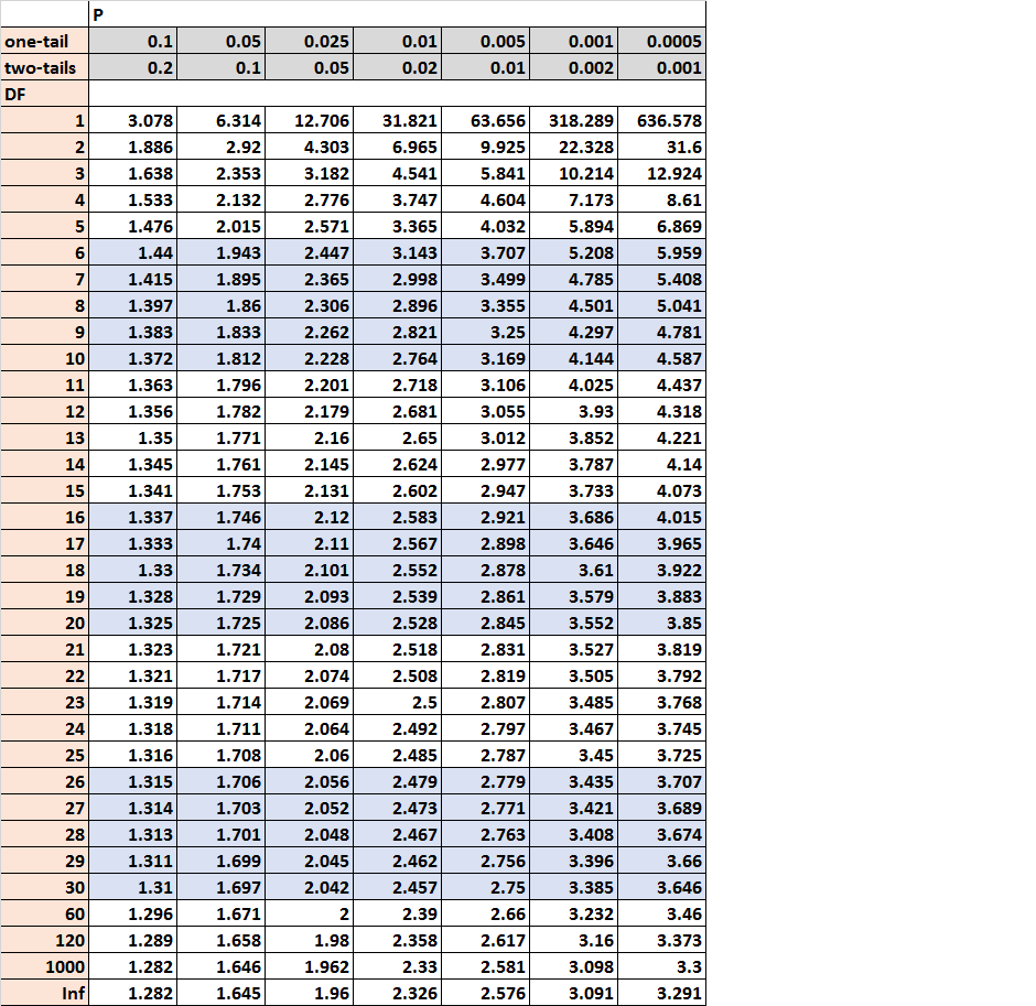
Lastly, would will find the t critical value in the t-distribution table that corresponds to a two-tailed test with alpha = .05 for 18 degrees of freedom:

The t critical value is 2.101.
We would then calculate our test statistic to be:
Test statistic: (x1 – x2) / (√s12/n1 + s22/n2)
Test statistic: (19.27 – 23.69) / (√20.42/11 + 83.23/13) = -4.42 / 2.873 = -1.538
Since the absolute value of our test statistic (1.538) is not larger than the t critical value, we fail to reject the null hypothesis of the test.
There is not sufficient evidence to say that the means of the two populations are significantly different.
The Satterthwaite Approximation in Practice
In practice, you will rarely have to calculate the Satterthwaite approximation by hand.
Instead, common statistical software like R, Python, Excel, SAS, and Stata can all use the Satterthwaite approximation to calculate the effective degrees of freedom automatically for you.
Additional Resources
Introduction to Hypothesis Testing
An Introduction to the Two Sample t-test
An Introduction to Welch’s t-test