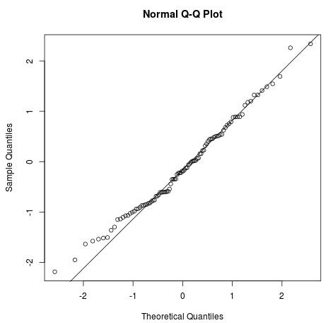
A Q-Q plot, short for “quantile-quantile” plot, is a type of plot that we can use to determine whether or not a set of data potentially came from some theoretical distribution.
Many statistical tests make the assumption that a set of data follows a normal distribution, and a Q-Q plot is often used to assess whether or not this assumption is met.
Although a Q-Q plot isn’t a formal statistical test, it does provide an easy way to visually check whether a dataset follows a normal distribution, and if not, how this assumption is violated and which data points potentially cause this violation.
We can create a Q-Q plot by plotting two sets of quantiles against one another. If both sets of quantiles came from the same distribution, then the points on the plot should roughly form a straight diagonal line.
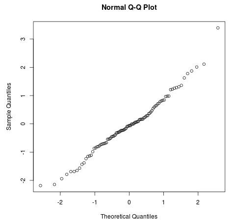
Quantiles represent points in a dataset below which a certain portion of the data fall. For example, the 0.9 quantile represents the point below which 90% of the data fall below. The 0.5 quantile represents the point below which 50% of the data fall below, and so on.
Q-Q plots identify the quantiles in your sample data and plot them against the quantiles of a theoretical distribution. In most cases the normal distribution is used, but a Q-Q plot can actually be created for any theoretical distribution.
If the data points fall along a straight diagonal line in a Q-Q plot, then the dataset likely follows a normal distribution.
How to Create a Q-Q Plot in R
We can easily create a Q-Q plot to check if a dataset follows a normal distribution by using the built-in qqnorm() function.
For example, the following code generates a vector of 100 random values that follow a normal distribution and creates a Q-Q plot for this dataset to verify that it does indeed follow a normal distribution:
#make this example reproducible
set.seed(11)

#generate vector of 100 values that follows a normal distribution
data #create Q-Q plot to compare this dataset to a theoretical normal distribution
qqnorm(data)
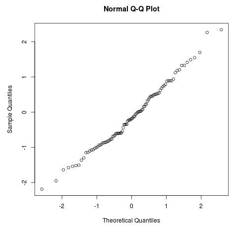
To make it even easier to see if the data falls along a straight line, we can use the qqline() function:
#create Q-Q plot
qqnorm(data)

#add straight diagonal line to plot
qqline(data)
We can see that the data points near the tails don’t fall exactly along the straight line, but for the most part this sample data appears to be normally distributed (as it should be since we told R to generate the data from a normal distribution).
Consider instead the following code that generates a vector of 100 random values that follow a gamma distribution and creates a Q-Q plot for this data to check if it follows a normal distribution:
#make this example reproducible
set.seed(11)

#generate vector of 100 values that follows a gamma distribution
data #create Q-Q plot to compare this dataset to a theoretical normal distribution
qqnorm(data)
qqline(data)
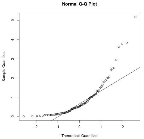
We can see the clear departure from the straight line in this Q-Q plot, indicating that this dataset likely does not follow a normal distribution.
Consider another chunk of code that generates a vector of 100 random values that follow a Chi-Square distribution with 5 degrees of freedom and creates a Q-Q plot for this data to check if it follows a normal distribution:
#make this example reproducible
set.seed(11)

#generate vector of 100 values that follows a Chi-Square distribution
data #create Q-Q plot to compare this dataset to a theoretical normal distribution
qqnorm(data)
qqline(data)
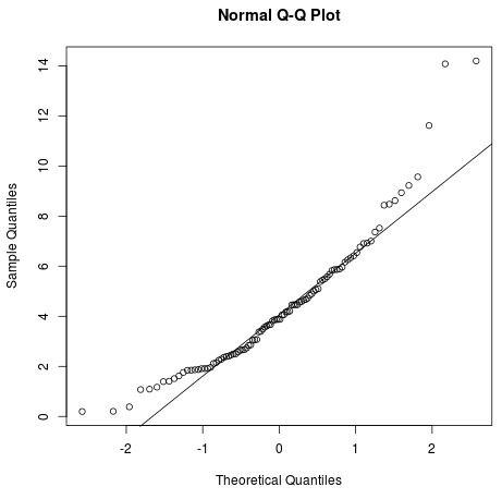
Once again we can see that this dataset does not appear to follow a normal distribution, especially near the tails.
Modifying the Aesthetics of a Q-Q Plot in R
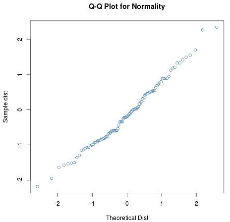
We can modify some of the aesthetics of the Q-Q plot in R including the title, axis labels, data point colors, line color, and line width.
The following code modifies the titles, axis labels, and color of the points in the plot:
#make this example reproducible
set.seed(11)

#generate vector of 100 values that follows a normal distribution
data #create Q-Q plot
qqnorm(data, main = 'Q-Q Plot for Normality', xlab = 'Theoretical Dist',
       ylab = 'Sample dist', col = 'steelblue')
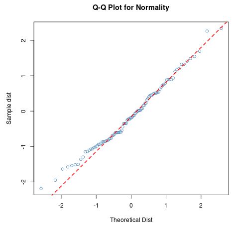
Next, the following code adds a straight diagonal line to the plot with a color of red, a line width of 2 (lwd = 2, default is 1), and a dashed line (lty = 2, default is 1):
qqline(data, col = 'red', lwd = 2, lty = 2)
Technical Notes
Keep in mind that a Q-Q plot is simply a way to visually check if a dataset follows a theoretical distribution. To formally test whether or not a dataset follows a particular distribution, the following tests can be performed (assuming you’re comparing your dataset to a normal distribution):
Anderson-Darling Test
Shapiro-Wilk Test
Kolmogorov-Smirnov Test
