Similar to a bar chart, a lollipop chart is useful for comparing the quantitative values of a categorical variable. Instead of using bars, though, a lollipop chart uses lines with circles on the end to represent the quantitative values.
A lollipop chart is an excellent way to compare multiple categories while keeping the amount of color on the chart minimal and drawing the attention of the reader to the actual values on the chart as opposed to the lines or other graphics on the chart. Many people also consider the lollipop chart to be aesthetically pleasing.
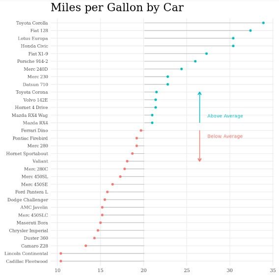
In this tutorial we will walk through the necessary steps to create the following lollipop chart:

Example: Lollipop Chart in R
For this example, we will use the built-in R dataset mtcars:
#view first six rows of mtcars
head(mtcars)
A Basic Lollipop Chart
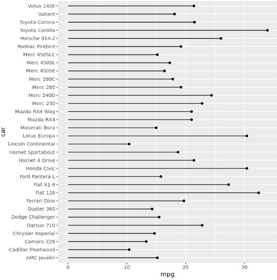
The following code illustrates how to create a lollipop chart to compare the mpg (miles per gallon) for each of the 32 cars in the dataset.
The names of the cars are defined in the row names of the dataset, so first we create a new column in the dataset that contains these row names.
Next, we load the library ggplot2, which we will use to actually create the lollipop chart.
With ggplot2, we use geom_segment to create the lines on the plot. We define the starting and ending x-values as 0 and mpg, respectively. We define the starting and ending y-values as car:
#create new column for car names
mtcars$car #load ggplot2 library
library(ggplot2)

#create lollipop chart
ggplot(mtcars, aes(x = mpg, y = car)) +
        geom_segment(aes(x = 0, y = car, xend = mpg, yend = car)) +
        geom_point()
Adding Labels
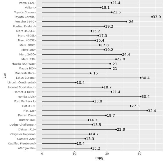
We can also add labels to the chart by using the label and geom_text arguments:
ggplot(mtcars, aes(x = mpg, y = car, label = mpg)) +
        geom_segment(aes(x = 0, y = car, xend = mpg, yend = car)) +
        geom_point() +
        geom_text(nudge_x = 1.5)
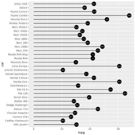
Or instead of placing the labels at the end of each line, we could place them inside of the circles themselves by enlarging the circles and changing the label font color to white:
ggplot(mtcars, aes(x = mpg, y = car, label = mpg)) +
        geom_segment(aes(x = 0, y = car, xend = mpg, yend = car)) +
        geom_point(size = 7) +
        geom_text(color = 'white', size = 2)
Comparing Values to an Average
We can also use a lollipop chart to compare values to a specific number. For example, we can find the average value for mpg in the dataset and then compare the mpg of each car to the average.
The following code uses the library dplyr to find the average value for mpg and then arrange the cars in order by mpg ascending:
#load library dplyr
library(dplyr)

#find mean value of mpg and arrange cars in order by mpg descending
mtcars_new %
                arrange(mpg) %>%
                mutate(mean_mpg = mean(mpg),
                       flag = ifelse(mpg - mean_mpg > 0, TRUE, FALSE),
                       car = factor(car, levels = .$car))

#view first six rows of mtcars_new
head(mtcars_new)

Next, the following code creates the lollipop chart by defining the color of the circle to be equal to the value of flag (in this case, TRUE or FALSE) and the starting x-value for each car is equal to the average value of mpg.
ggplot(mtcars_new, aes(x = mpg, y = car, color = flag)) +
        geom_segment(aes(x = mean_mpg, y = car, xend = mpg, yend = car)) +
        geom_point()
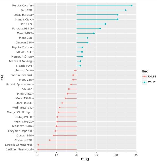
By using this type of color scheme, we can easily tell which cars have an mpg less than and above the average for the dataset.
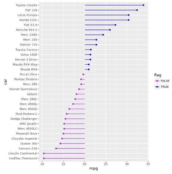
By default, R uses blue and red as the colors for the chart. However, we can use whatever colors we’d like by using the scale_colour_manual argument:
ggplot(mtcars_new, aes(x = mpg, y = car, color = flag)) +
        geom_segment(aes(x = mean_mpg, y = car, xend = mpg, yend = car)) +
        geom_point() +
        scale_colour_manual(values = c("purple", "blue"))
Altering the Aesthetics of the Chart
Lastly, we can use the wide capabilities of ggplot2 to alter the aesthetics of the chart further and create a professional-looking final product:
ggplot(mtcars_new, aes(x = mpg, y = car, color = flag)) +
        geom_segment(aes(x = mean_mpg, y = car, xend = mpg, yend = car), color = "grey") +
        geom_point() +
        annotate("text", x = 27, y = 20, label = "Above Average", color = "#00BFC4", size = 3, hjust = -0.1, vjust = .75) +
        annotate("text", x = 27, y = 17, label = "Below Average", color = "#F8766D", size = 3, hjust = -0.1, vjust = -.1) +
        geom_segment(aes(x = 26.5, xend = 26.5, y = 19, yend = 23),
                     arrow = arrow(length = unit(0.2,"cm")), color = "#00BFC4") +
        geom_segment(aes(x = 26.5, xend = 26.5 , y = 18, yend = 14),
                     arrow = arrow(length = unit(0.2,"cm")), color = "#F8766D") +
        labs(title = "Miles per Gallon by Car") +
        theme_minimal() +
        theme(axis.title = element_blank(),
              panel.grid.minor = element_blank(),
              legend.position = "none",
              text = element_text(family = "Georgia"),
              axis.text.y = element_text(size = 8),
              plot.title = element_text(size = 20, margin = margin(b = 10), hjust = 0),
              plot.subtitle = element_text(size = 12, color = "darkslategrey", margin = margin(b = 25, l = -25)),
              plot.caption = element_text(size = 8, margin = margin(t = 10), color = "grey70", hjust = 0))
