Often you may want to use VLOOKUP in Google Sheets to look up values based on multiple criteria.
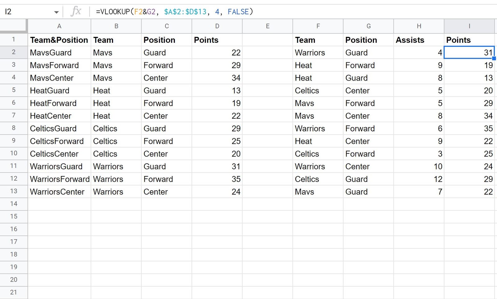
For example, suppose we have the following two datasets and you would like to use VLOOKUP in the right dataset to return the value in the Points column that matches both the value in the Team column and the Position column in the left dataset:

The following step-by-step example shows how to do so.
Step 1: Create a Helper Column
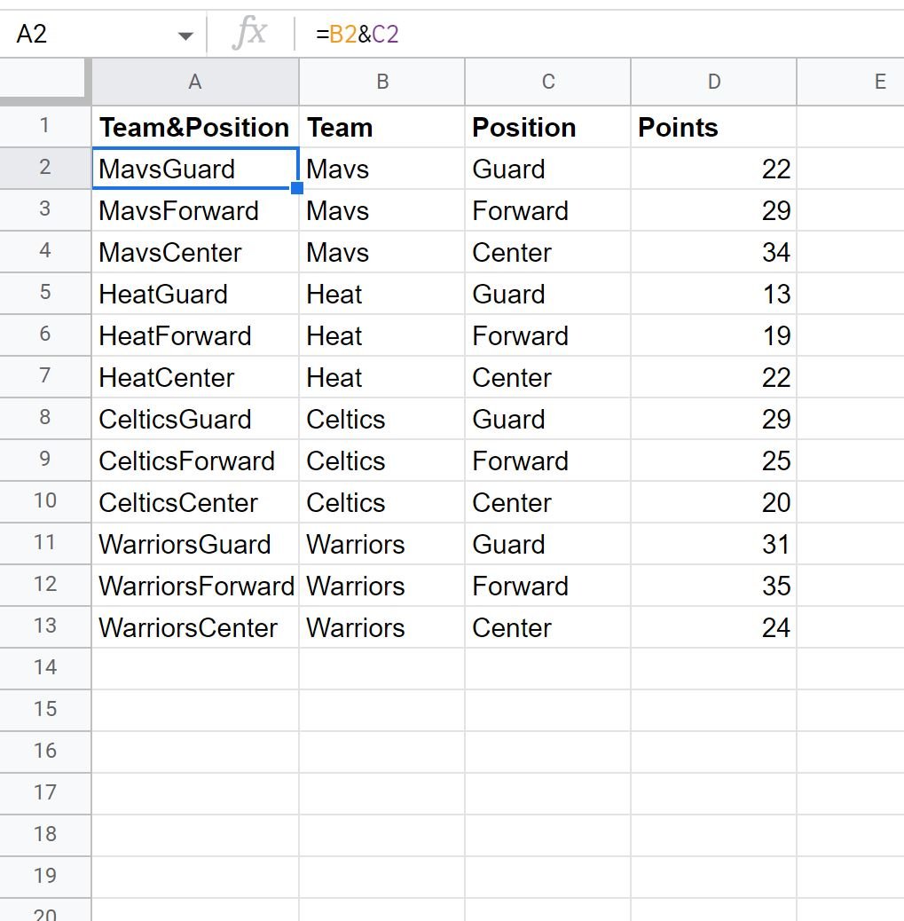
Before we can perform the VLOOKUP, we must first create a helper column in the first dataset that joins together the values in the Team and Points columns.
We’ll type the following formula into cell A2:
=B2&C2
We’ll then drag and fill this formula down to each remaining cell in column A:

Column A now contains a concatenation of the Team and Position values.
We will use this new column in our VLOOKUP formula in the next step.
Step 2: Use VLOOKUP with Multiple Criteria
Next, we can type the following formula into cell I2:
=VLOOKUP(F2&G2, $A$2:$D$13, 4, FALSE)
We’ll then drag and fill this formula down to each remaining cell in column I:

This formula looks up the concatenation of the text values in columns F and G in column A and returns the corresponding value in column D.
Notice that the points value for each player in the right dataset matches the points value for the corresponding player in the left dataset.
We have successfully used a VLOOKUP with multiple criteria.
Additional Resources
The following tutorials explain how to perform other common operations in Google Sheets:
How to Use IFERROR with VLOOKUP in Google Sheets
How to Perform a Reverse VLOOKUP in Google Sheets
How to Use a Case Sensitive VLOOKUP in Google Sheets