Often you may want to apply conditional formatting to cells whose values fall between two specific values in Excel.
The following example shows exactly how to do so.
Example: Conditional Formatting if Between Two Values
Suppose we have the following dataset that contains information about various basketball teams:

Suppose we would like to highlight each value in the points column where the value is between 10 and 20.
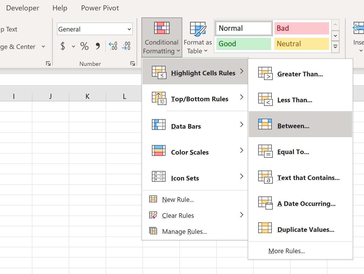
To do so, highlight the values in the range B2:B14, then click the Conditional Formatting icon on the Home tab, then click Highlight Cells Rules, then Between:

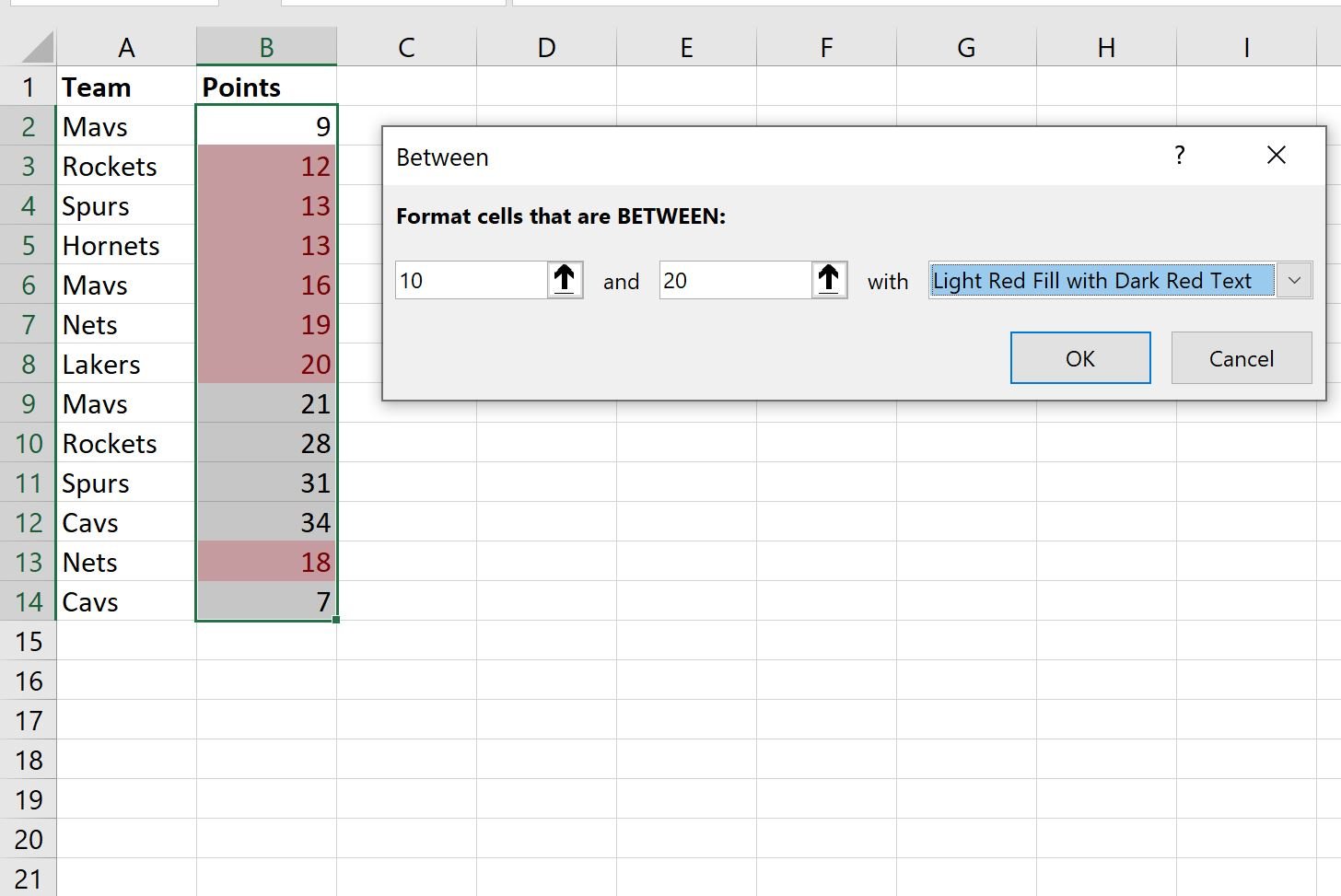
In the new window that appears, choose 10 as the lower value and 20 as the upper value:

One you click OK, the values in the points column that fall between 10 and 20 will automatically be formatted with a light red background and dark red text:

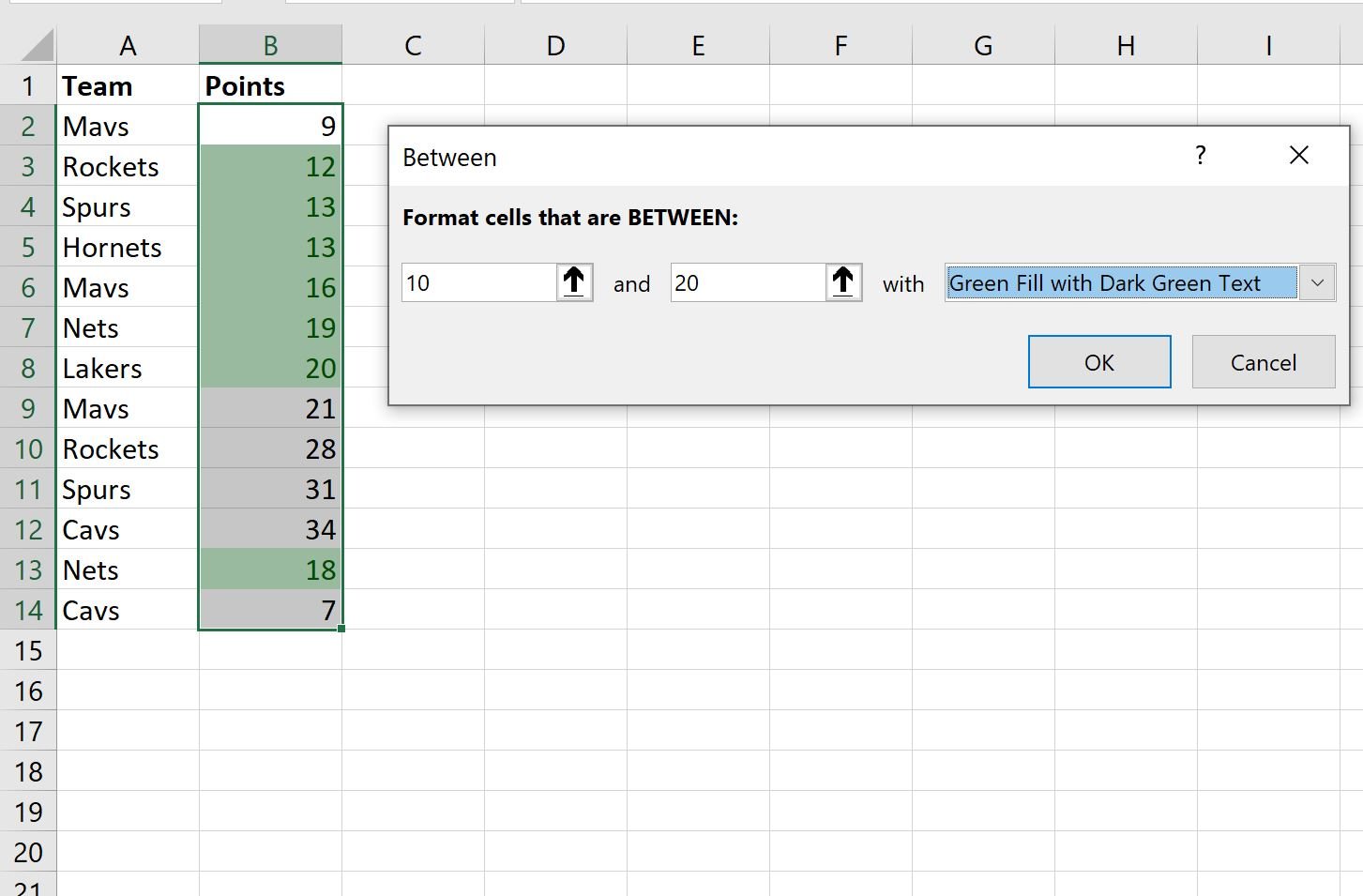
Note that you can also choose a different format for the cells.
For example, you could choose to format the cells using a green background with dark green text:

You can also choose Custom Format to specify a custom format style for the cells:

This allows you to pick any combination of styles you’d like for the background color and text color.
Additional Resources
The following tutorials explain how to perform other common tasks in Excel:
How to Apply Conditional Formatting if Cell Contains Text in Excel
How to Apply Conditional Formatting with Multiple Conditions in Excel