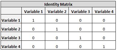
Bartlett’s Test of Sphericity compares an observed correlation matrix to the identity matrix. Essentially it checks to see if there is a certain redundancy between the variables that we can summarize with a few number of factors.
The null hypothesis of the test is that the variables are orthogonal, i.e. not correlated. The alternative hypothesis is that the variables are not orthogonal, i.e. they are correlated enough to where the correlation matrix diverges significantly from the identity matrix.
This test is often performed before we use a data reduction technique such as principal component analysis or factor analysis to verify that a data reduction technique can actually compress the data in a meaningful way.
Note: Bartlett’s Test of Sphericity is not the same as Bartlett’s Test for Equality of Variances. This is a common confusion, since the two have similar names.
Correlation Matrix vs. Identity Matrix
A correlation matrix is simply a matrix of values that shows the correlation coefficients between variables. For example, the following correlation matrix shows the correlation coefficients between different variables for professional basketball teams.

Correlation coefficients can vary from -1 to 1. The further a value is from 0, the higher the correlation between two variables.
An identity matrix is a matrix in which all of the values along the diagonal are 1 and all of the other values are 0.

In this case, if the numbers in this matrix represent correlation coefficients it means that each variable is perfectly orthogonal (i.e. “uncorrelated”) to every other variable and thus a data reduction technique like PCA or factor analysis would not be able to “compress” the data in any meaningful way.
Thus, the reason we conduct Bartlett’s Test of Sphericity is to make sure that the correlation matrix of the variables in our dataset diverges significantly from the identity matrix, so that we know a data reduction technique is suitable to use.
If the p-value from Bartlett’s Test of Sphericity is lower than our chosen significance level (common choices are 0.10, 0.05, and 0.01), then our dataset is suitable for a data reduction technique.
How to Conduct Bartlett’s Test of Sphericity in R
To conduct Bartlett’s Test of Sphericity in R, we can use the cortest.bartlett() function from the psych library. The general syntax for this function is as follows:
cortest.bartlett(R, n)
- R: a correlation matrix of the dataset
- n: sample size of the dataset
The following code illustrates how to conduct this test on a fake dataset we created:
#make this example reproducible
set.seed(0)

#create fake data
data #view first six rows of data
head(data)
#           A          B           C
#1  6.0518171  4.5968242 11.25487348
#2 -0.3049334  0.7397837 -1.21421297
#3  6.3191971 17.6481878  0.07208074
#4  6.0897173 -1.7720347  5.37264242
#5  2.6585657  2.6707352 -4.04308622
#6 -5.1598002  4.5008479  9.61375026

#find correlation matrix of data
cor_matrix #view correlation matrix
cor_matrix

#          A            B            C
#A 1.0000000 0.1600155667 0.2825308511
#B 0.1600156 1.0000000000 0.0005358384
#C 0.2825309 0.0005358384 1.0000000000

#load psych library
library(psych)

#perform Bartlett's Test of Sphericity
cortest.bartlett(cor_matrix, n = nrow(data))

#$chisq
#[1] 5.252329
#
#$p.value
#[1] 0.1542258
#
#$df
#[1] 3
The Chi-Square test statistic is 5.252329 and the corresponding p-value is 0.1542258, which is not smaller than our significance level (let’s use 0.05). Thus, this data is likely not suitable for PCA or factor analysis.
To put this in layman’s terms, the three variables in our dataset are fairly uncorrelated so a data reduction technique like PCA or factor analysis would have a hard time compressing these variables into linear combinations that are able to capture significant variance present in the data.