Many statistical tests make the assumption that datasets are normally distributed.
There are four common ways to check this assumption in R:
1. (Visual Method) Create a histogram.
- If the histogram is roughly “bell-shaped”, then the data is assumed to be normally distributed.
2. (Visual Method) Create a Q-Q plot.
- If the points in the plot roughly fall along a straight diagonal line, then the data is assumed to be normally distributed.
3. (Formal Statistical Test) Perform a Shapiro-Wilk Test.
- If the p-value of the test is greater than α = .05, then the data is assumed to be normally distributed.
4. (Formal Statistical Test) Perform a Kolmogorov-Smirnov Test.
- If the p-value of the test is greater than α = .05, then the data is assumed to be normally distributed.
The following examples show how to use each of these methods in practice.
Method 1: Create a Histogram
The following code shows how to create a histogram for a normally distributed and non-normally distributed dataset in R:
#make this example reproducible
set.seed(0)

#create data that follows a normal distribution
normal_data #create data that follows an exponential distribution
non_normal_data #define plotting region
par(mfrow=c(1,2))

#create histogram for both datasets
hist(normal_data, col='steelblue', main='Normal')
hist(non_normal_data, col='steelblue', main='Non-normal')
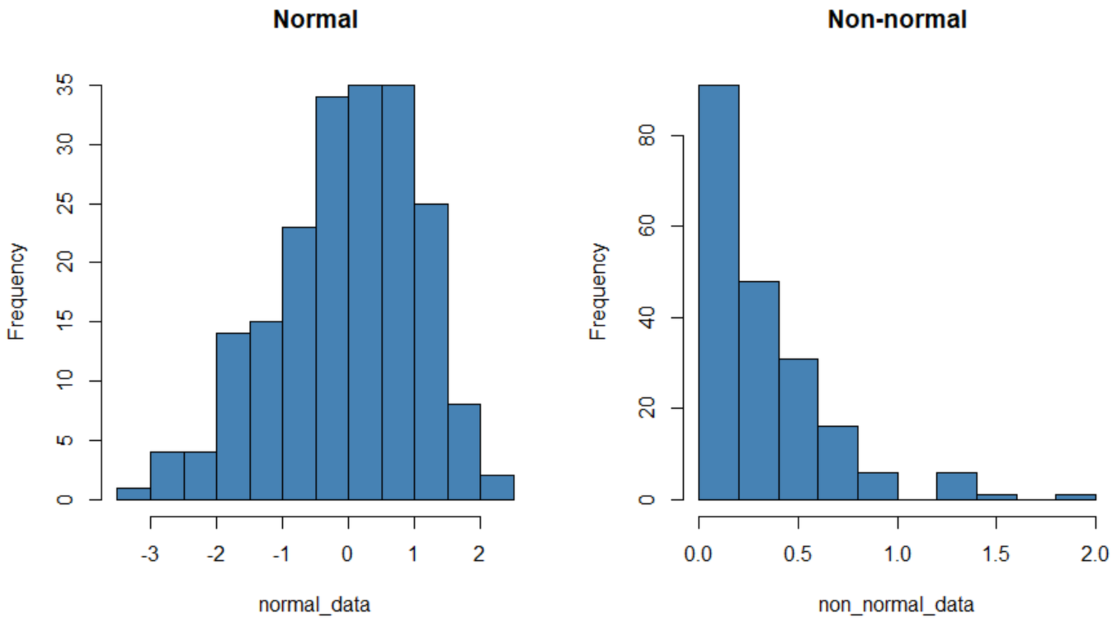
The histogram on the left exhibits a dataset that is normally distributed (roughly a “bell-shape”) and the one on the right exhibits a dataset that is not normally distributed.
Method 2: Create a Q-Q plot
The following code shows how to create a Q-Q plot for a normally distributed and non-normally distributed dataset in R:
#make this example reproducible
set.seed(0)

#create data that follows a normal distribution
normal_data #create data that follows an exponential distribution
non_normal_data #define plotting region
par(mfrow=c(1,2))

#create Q-Q plot for both datasets
qqnorm(normal_data, main='Normal')
qqline(normal_data)

qqnorm(non_normal_data, main='Non-normal')
qqline(non_normal_data)
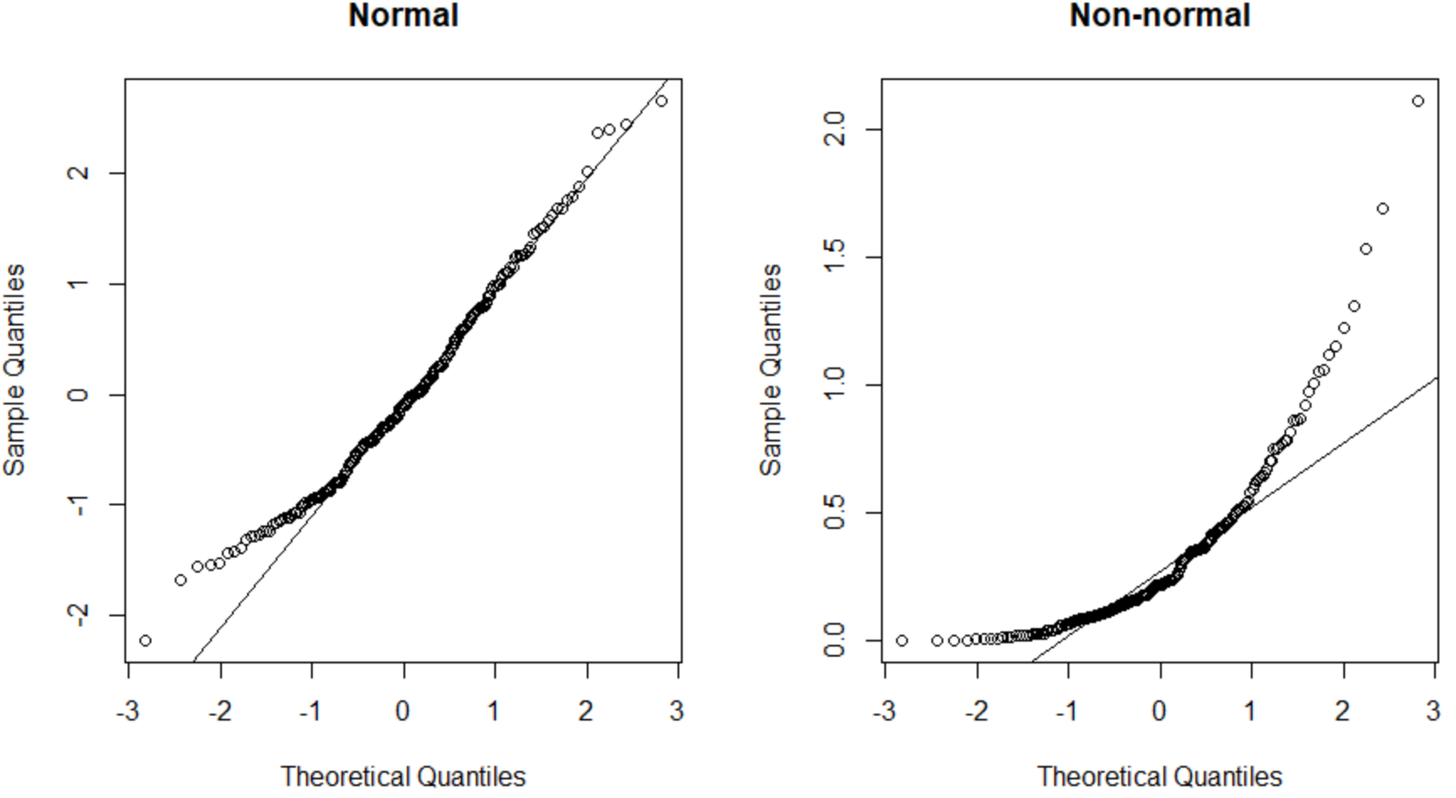
The Q-Q plot on the left exhibits a dataset that is normally distributed (the points fall along a straight diagonal line) and the Q-Q plot on the right exhibits a dataset that is not normally distributed.
Method 3: Perform a Shapiro-Wilk Test
The following code shows how to perform a Shapiro-Wilk test on a normally distributed and non-normally distributed dataset in R:
#make this example reproducible
set.seed(0)

#create data that follows a normal distribution
normal_data #perform shapiro-wilk test
shapiro.test(normal_data)

	Shapiro-Wilk normality test

data:  normal_data
W = 0.99248, p-value = 0.3952

#create data that follows an exponential distribution
non_normal_data #perform shapiro-wilk test
shapiro.test(non_normal_data)

	Shapiro-Wilk normality test

data:  non_normal_data
W = 0.84153, p-value = 1.698e-13
The p-value of the first test is not less than .05, which indicates that the data is normally distributed.
The p-value of the second test is less than .05, which indicates that the data is not normally distributed.
Method 4: Perform a Kolmogorov-Smirnov Test
The following code shows how to perform a Kolmogorov-Smirnov test on a normally distributed and non-normally distributed dataset in R:
#make this example reproducible
set.seed(0)

#create data that follows a normal distribution
normal_data #perform kolmogorov-smirnov test
ks.test(normal_data, 'pnorm')

	One-sample Kolmogorov-Smirnov test

data:  normal_data
D = 0.073535, p-value = 0.2296
alternative hypothesis: two-sided

#create data that follows an exponential distribution
non_normal_data #perform kolmogorov-smirnov test
ks.test(non_normal_data, 'pnorm')
	One-sample Kolmogorov-Smirnov test

data:  non_normal_data
D = 0.50115, p-value
The p-value of the first test is not less than .05, which indicates that the data is normally distributed.
The p-value of the second test is less than .05, which indicates that the data is not normally distributed.
How to Handle Non-Normal Data
If a given dataset is not normally distributed, we can often perform one of the following transformations to make it more normally distributed:
1. Log Transformation: Transform the values from x to log(x).
2. Square Root Transformation: Transform the values from x to √x.
3. Cube Root Transformation: Transform the values from x to x1/3.
By performing these transformations, the dataset typically becomes more normally distributed.
Read this tutorial to see how to perform these transformations in R.
Additional Resources
How to Create Histograms in R
How to Create & Interpret a Q-Q Plot in R
How to Perform a Shapiro-Wilk Test in R
How to Perform a Kolmogorov-Smirnov Test in R