A Complete Guide: The 2×2 Factorial Design

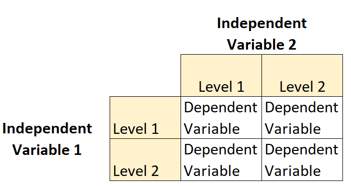
A 2×2 factorial design is a type of experimental design that allows researchers to understand the effects of two independent variables (each with two levels) on a single dependent variable.

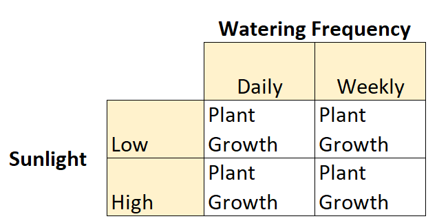
For example, suppose a botanist wants to understand the effects of sunlight (low vs. high) and watering frequency (daily vs. weekly) on the growth of a certain species of plant.

This is an example of a 2×2 factorial design because there are two independent variables, each with two levels:

• Independent variable #1: Sunlight
  • Levels: Low, High
• Independent variable #2: Watering Frequency
  • Levels: Daily, Weekly

And there is one dependent variable: Plant growth.

The Purpose of a 2×2 Factorial Design

A 2×2 factorial design allows you to analyze the following effects:

Main Effects: These are the effects that just one independent variable has on the dependent variable.

For example, in our previous scenario we could analyze the following main effects:

• Main effect of sunlight on plant growth.
  • We can find the mean plant growth of all plants that received low sunlight.
  • We can find the mean plant growth of all plants that received high sunlight.
• Main effect of watering frequency on plant growth.
  • We can find the mean plant growth of all plants that were watered daily.
  • We can find the mean plant growth of all plants that were watered weekly.

Interaction Effects: These occur when the effect that one independent variable has on the dependent variable depends on the level of the other independent variable.

For example, in our previous scenario we could analyze the following interaction effects:

• Does the effect of sunlight on plant growth depend on watering frequency?
• Does the effect of watering frequency on plant growth depend on the amount of sunlight?

Visualizing Main Effects & Interaction Effects

When we use a 2×2 factorial design, we often graph the means to gain a better understanding of the effects that the independent variables have on the dependent variable.

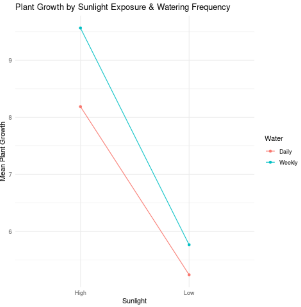
For example, consider the following plot:

Here’s how to interpret the values in the plot:

• The mean growth for plants that received high sunlight and daily watering was about 8.2 inches.
• The mean growth for plants that received high sunlight and weekly watering was about 9.6 inches.
• The mean growth for plants that received low sunlight and daily watering was about 5.3 inches.
• The mean growth for plants that received low sunlight and weekly watering was about 5.8 inches.

To determine if there is an interaction effect between the two independent variables, we simply need to inspect whether or not the lines are parallel:

• If the two lines in the plot are parallel, there is no interaction effect.
• If the two lines in the plot are not parallel, there is an interaction effect.

In the previous plot, the two lines were roughly parallel so there is likely no interaction effect between watering frequency and sunlight exposure.

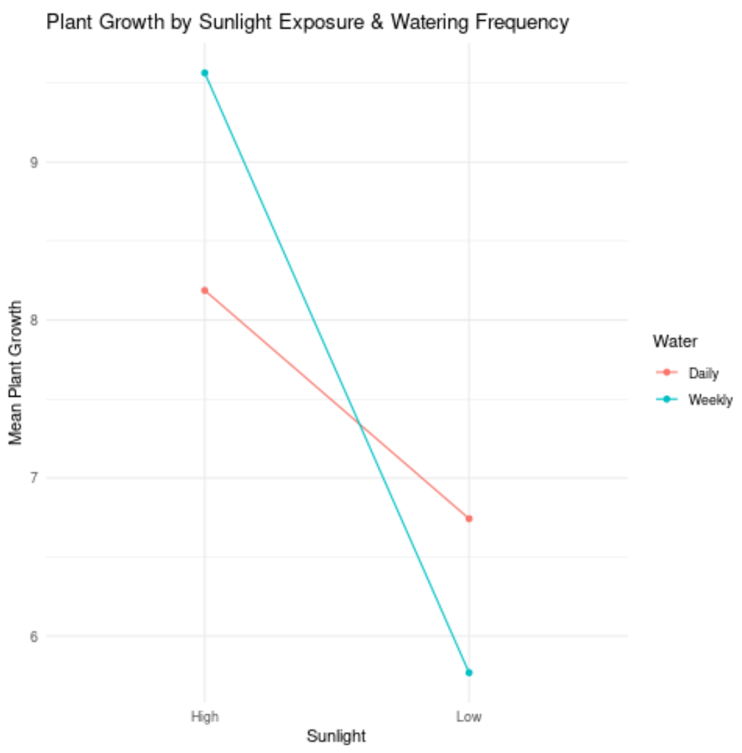
However, consider the following plot:

The two lines are not parallel at all (in fact, they cross!), which indicates that there is likely an interaction effect between them.

For example, this means the effect that sunlight has on plant growth depends on the watering frequency.

In other words, sunlight and watering frequency do not affect plant growth independently. Rather, there is an interaction effect between the two independent variables.

How to Analyze a 2×2 Factorial Design

Plotting the means is a visualize way to inspect the effects that the independent variables have on the dependent variable.

However, we can also perform a two-way ANOVA to formally test whether or not the independent variables have a statistically significant relationship with the dependent variable.

For example, the following code shows how to perform a two-way ANOVA for our hypothetical plant scenario in R:

#make this example reproducible
set.seed(0)

df frame(sunlight = rep(c('Low', 'High'), each = 30),
                 water = rep(c('Daily', 'Weekly'), each = 15, times = 2),
                 growth = c(rnorm(15, 6, 2), rnorm(15, 7, 3), rnorm(15, 7, 2),
                                   rnorm(15, 10, 3)))

#fit the two-way ANOVA model
model #view the model output
summary(model)

               Df Sum Sq Mean Sq F value  Pr(>F)   
sunlight        1   52.5   52.48   8.440 0.00525 **
water           1   31.6   31.59   5.081 0.02813 * 
sunlight:water  1   12.8   12.85   2.066 0.15620   
Residuals      56  348.2    6.22                   
---
Signif. codes:  0 ‘***’ 0.001 ‘**’ 0.01 ‘*’ 0.05 ‘.’ 0.1 ‘ ’ 1

Here’s how to interpret the output of the ANOVA:

• The p-value associated with sunlight is .005. Since this is less than .05, this means sunlight exposure has a statistically significant effect on plant growth.
• The p-value associated with water is .028. Since this is less than .05, this means watering frequency also has a statistically significant effect on plant growth.
• The p-value for the interaction between sunlight and water is .156. Since this is not less than .05, this means there is no interaction effect between sunlight and water.

Additional Resources

A Complete Guide: The 2×3 Factorial Design
What Are Levels of an Independent Variable?
Independent vs. Dependent Variables
What is a Factorial ANOVA?