A one-way ANOVA is used to determine whether or not there is a statistically significant difference between the means of three or more independent groups.
If the overall p-value from the ANOVA table is less than some significance level, then we have sufficient evidence to say that at least one of the means of the groups is different from the others.
However, this doesn’t tell us which groups are different from each other. It simply tells us that not all of the group means are equal.
In order to find out exactly which groups are different from each other, we must conduct a post-hoc test that is capable of controlling the family-wise error rate.
One of the most commonly used post hoc tests is Scheffe’s test.
This tutorial explains how to perform Scheffe’s test in R.
Example: Scheffe’s Test in R
Suppose a teacher wants to know whether or not three different studying techniques lead to different exam scores among students. To test this, she randomly assigns 10 students to use each studying technique and records their exam scores.
We can use the following steps in R to fit a one-way ANOVA to test for differences in mean exam scores among the three groups and use Scheffe’s test to determine exactly which groups are different.
Step 1: Create the dataset.
The following code shows how to create a dataset that contains exam scores for all 30 students:
#create data frame
data rep(c("tech1", "tech2", "tech3"), each = 10),
                   score = c(76, 77, 77, 81, 82, 82, 83, 84, 85, 89,
                             81, 82, 83, 83, 83, 84, 87, 90, 92, 93,
                             77, 78, 79, 88, 89, 90, 91, 95, 95, 98))

#view first six rows of data frame
head(data)

  technique score
1     tech1    76
2     tech1    77
3     tech1    77
4     tech1    81
5     tech1    82
6     tech1    82
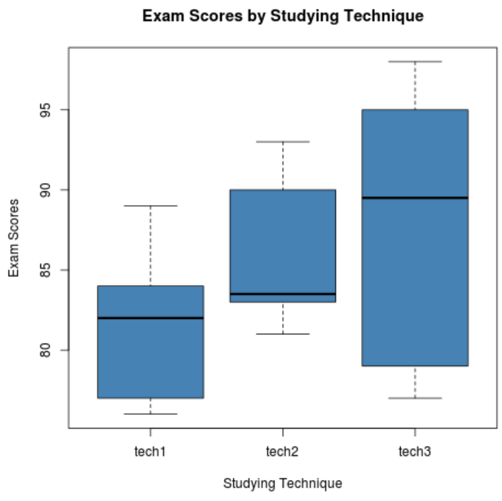
Step 2: Visualize the exam scores for each group.
The following code shows how to produce boxplots to visualize the distribution of exam scores for each group:
boxplot(score ~ technique,
        data = data,
        main = "Exam Scores by Studying Technique",
        xlab = "Studying Technique",
        ylab = "Exam Scores",
        col = "steelblue",
        border = "black")

Step 3: Perform a one-way ANOVA.
The following code shows how to perform a one-way ANOVA to test for differences among mean exam scores in each group:
#fit the one-way ANOVA model
model #view model output
summary(model)

            Df Sum Sq Mean Sq F value Pr(>F)
technique    2  211.5  105.73   3.415 0.0476 *
Residuals   27  836.0   30.96
---
Signif. codes:  0 '***' 0.001 '**' 0.01 '*' 0.05 '.' 0.1 ' ' 1
Since the overall p-value (0.0476) is less than .05, this is an indication that each group does not have the same average exam score.
Next, we will perform Scheffe’s test to determine which groups are different.
Step 4: Perform Scheffe’s Test.
To perform Scheffe’s test, we’ll use the ScheffeTest() function from the DescTools package.
The following code shows how to use this function for our example:
#load DescTools package
library(DescTools)

#perform Scheffe's test
ScheffeTest(model)

  Posthoc multiple comparisons of means : Scheffe Test
    95% family-wise confidence level

$technique
            diff      lwr.ci    upr.ci   pval
tech2-tech1  4.2 -2.24527202 10.645272 0.2582
tech3-tech1  6.4 -0.04527202 12.845272 0.0519 .
tech3-tech2  2.2 -4.24527202  8.645272 0.6803

---
Signif. codes:  0 '***' 0.001 '**' 0.01 '*' 0.05 '.' 0.1 ' ' 1
The way to interpret the output is as follows:
- The mean difference in exam scores between technique 2 and technique 1 is 4.2. The corresponding p-value for the mean difference is .2582.
- The mean difference in exam scores between technique 3 and technique 1 is 6.4. The corresponding p-value for the mean difference is .0519.
- The mean difference in exam scores between technique 3 and technique 2 is 2.2. The corresponding p-value for the mean difference is .6803.
Depending on the significance level we decide to use, the only two groups that seem to be statistically significantly different are technique 3 and technique 1.
Additional Resources
How to Conduct a One-Way ANOVA in R
How to Perform Tukey’s Test in R
How to Perform a Bonferroni Correction in R