A residual is the difference between an observed value and a predicted value in regression analysis.
It is calculated as:
Residual = Observed value – Predicted value
Recall that the goal of linear regression is to quantify the relationship between one or more predictor variables and a response variable. To do this, linear regression finds the line that best “fits” the data, known as the least squares regression line.
This line produces a prediction for each observation in the dataset, but it’s unlikely that the prediction made by the regression line will exactly match the observed value.
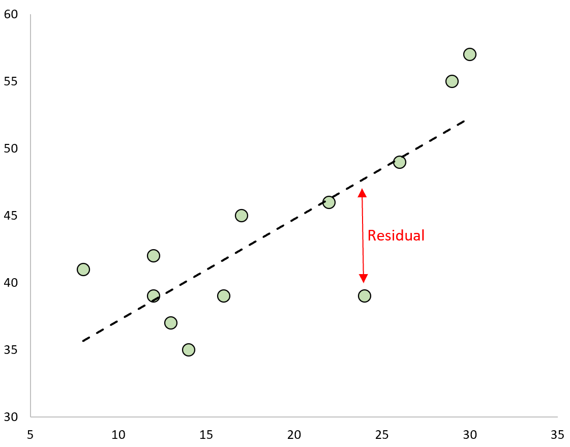
The difference between the prediction and the observed value is the residual. If we plot the observed values and overlay the fitted regression line, the residuals for each observation would be the vertical distance between the observation and the regression line:
An observation has a positive residual if its value is greater than the predicted value made by the regression line.
Conversely, an observation has a negative residual if its value is less than the predicted value made by the regression line.
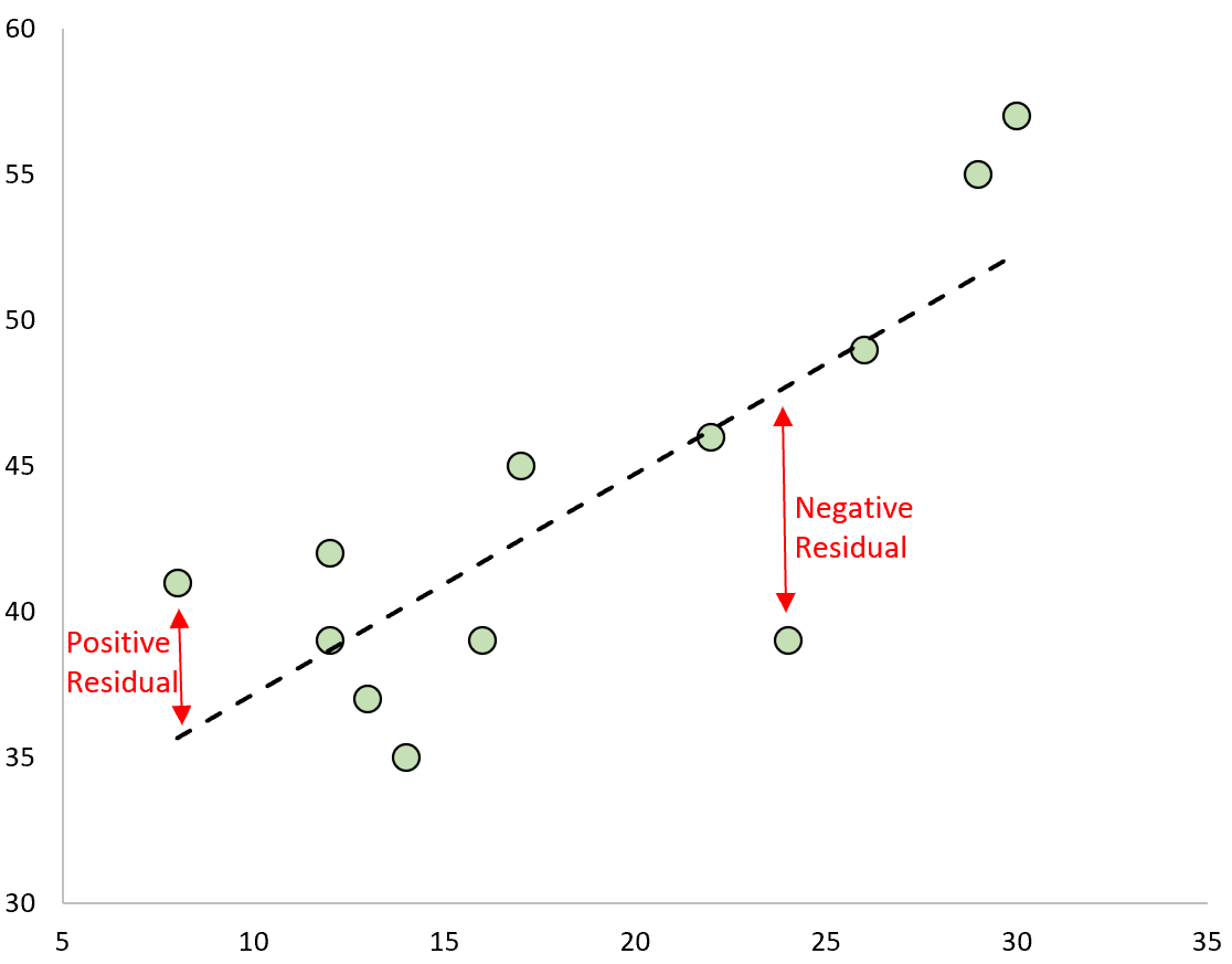
Some observations will have positive residuals while others will have negative residuals, but all of the residuals will add up to zero.
Example of Calculating Residuals
Suppose we have the following dataset with 12 total observations:

If we use some statistical software (like R, Excel, Python, Stata, etc.) to fit a linear regression line to this dataset, we’ll find that the line of best fit turns out to be:
y = 29.63 + 0.7553x
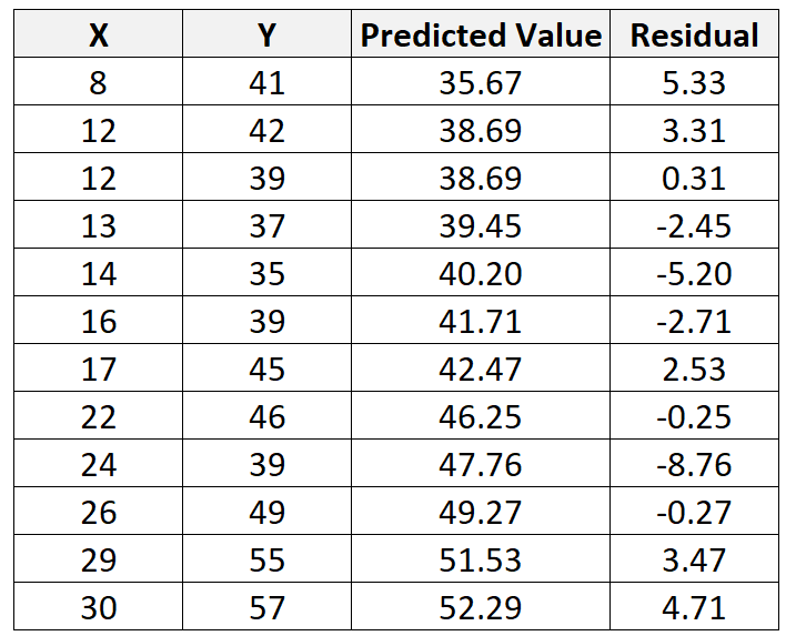
Using this line, we can calculate the predicted value for each Y value based on the value of X. For example, the predicted value of the first observation would be:
y = 29.63 + 0.7553*(8) = 35.67
We can then calculate the residual for this observation as:
Residual = Observed value – Predicted value = 41 – 35.67 = 5.33
We can repeat this process to find the residual for every single observation:
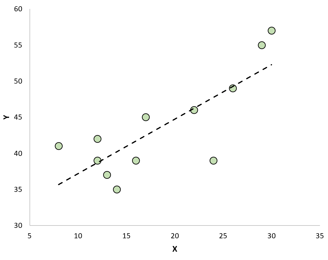
If we create a scatterplot to visualize the observations along with the fitted regression line, we’ll see that some of the observations lie above the line while some fall below the line:
Properties of Residuals
Residuals have the following properties:
- Each observation in a dataset has a corresponding residual. So, if a dataset has 100 total observations then the model will produce 100 predicted values, which results in 100 total residuals.
- The sum of all residuals adds up to zero.
- The mean value of the residuals is zero.
How Are Residuals Used in Practice?
In practice, residuals are used for three different reasons in regression:
1. Assess model fit.
Once we produce a fitted regression line, we can calculate the residuals sum of squares (RSS), which is the sum of all of the squared residuals. The lower the RSS, the better the regression model fits the data.
2. Check the assumption of normality.
One of the key assumptions of linear regression is that the residuals are normally distributed.
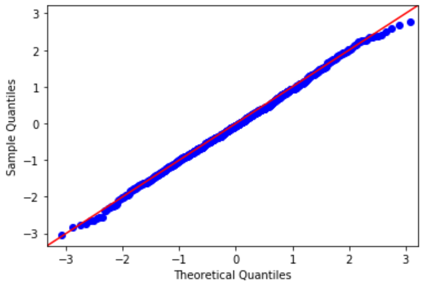
To check this assumption, we can create a Q-Q plot, which is a type of plot that we can use to determine whether or not the residuals of a model follow a normal distribution.
If the points on the plot roughly form a straight diagonal line, then the normality assumption is met.
3. Check the assumption of homoscedasticity.
Another key assumption of linear regression is that the residuals have constant variance at every level of x. This is known as homoscedasticity. When this is not the case, the residuals are said to suffer from heteroscedasticity.
To check if this assumption is met, we can create a residual plot, which is a scatterplot that shows the residuals vs. the predicted values of the model.
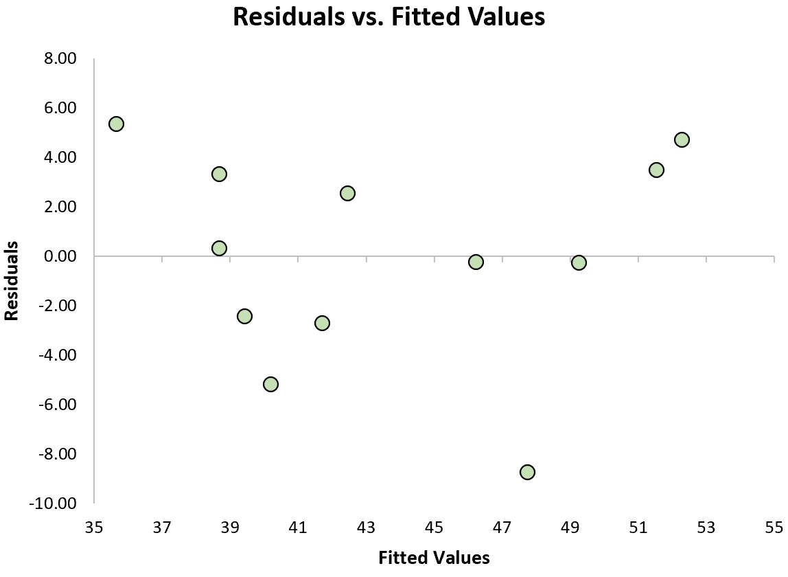
If the residuals are roughly evenly scattered around zero in the plot with no clear pattern, then we typically say the assumption of homoscedasticity is met.
Additional Resources
Introduction to Simple Linear Regression
Introduction to Multiple Linear Regression
The Four Assumptions of Linear Regression
How to Create a Residual Plot in Excel