Often you may want to select a random sample from a dataset in Excel. Fortunately this is easy to do using the RAND() function, which generates a random number between 0 and 1.
This tutorial provides a step-by-step example of how to use this function to select a random sample in Excel.
Step 1: Create a Dataset
First, enter the values of your dataset into a single column. For this example, we’ll enter 20 different values in column A:

Step 2: Create a List of Random Values
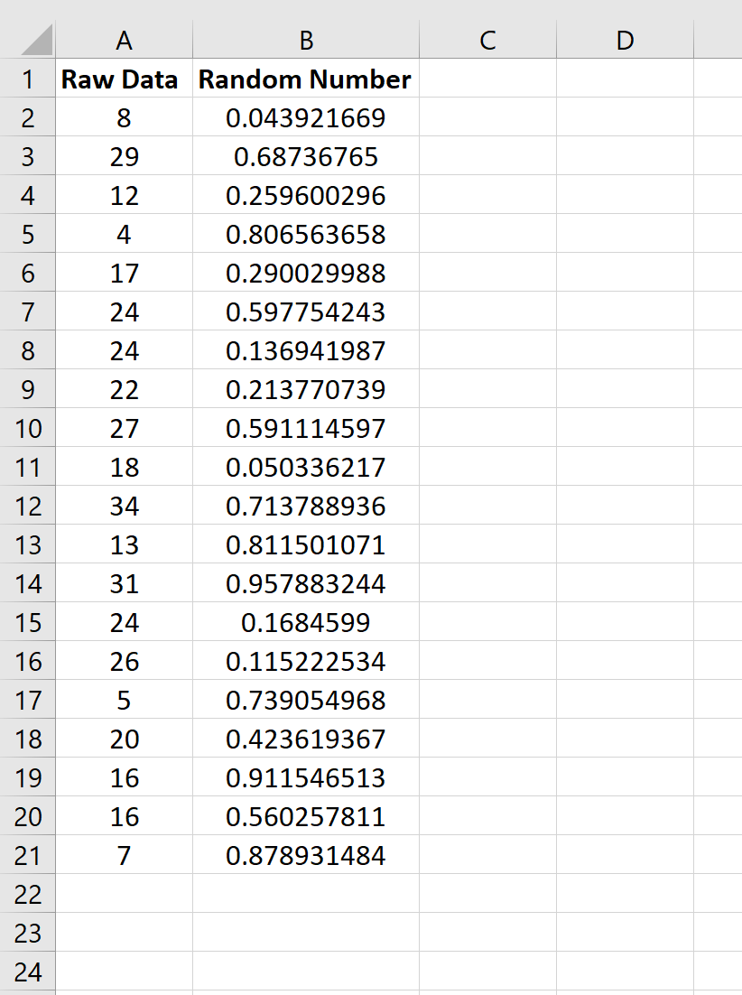
Next, type =RAND() into cell B2. This creates a random value between 0 and 1.
Next, hover over the bottom right corner of cell B2 until a tiny + appears and then double click. This will copy the =RAND() formula down to all of the remaining cells in column B:
Step 3: Copy & Paste the Random Values
Next, highlight the values in column B and click Ctrl + C. This will copy all of the values. Next, right click on cell C2 and choose Paste Values.
Note that the values in column B may change once you do this, but don’t worry about this.
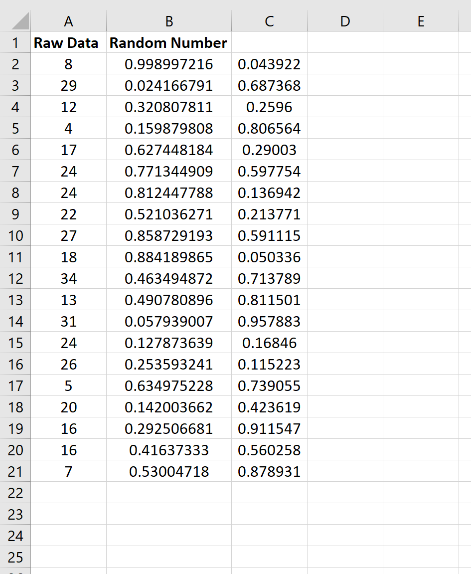
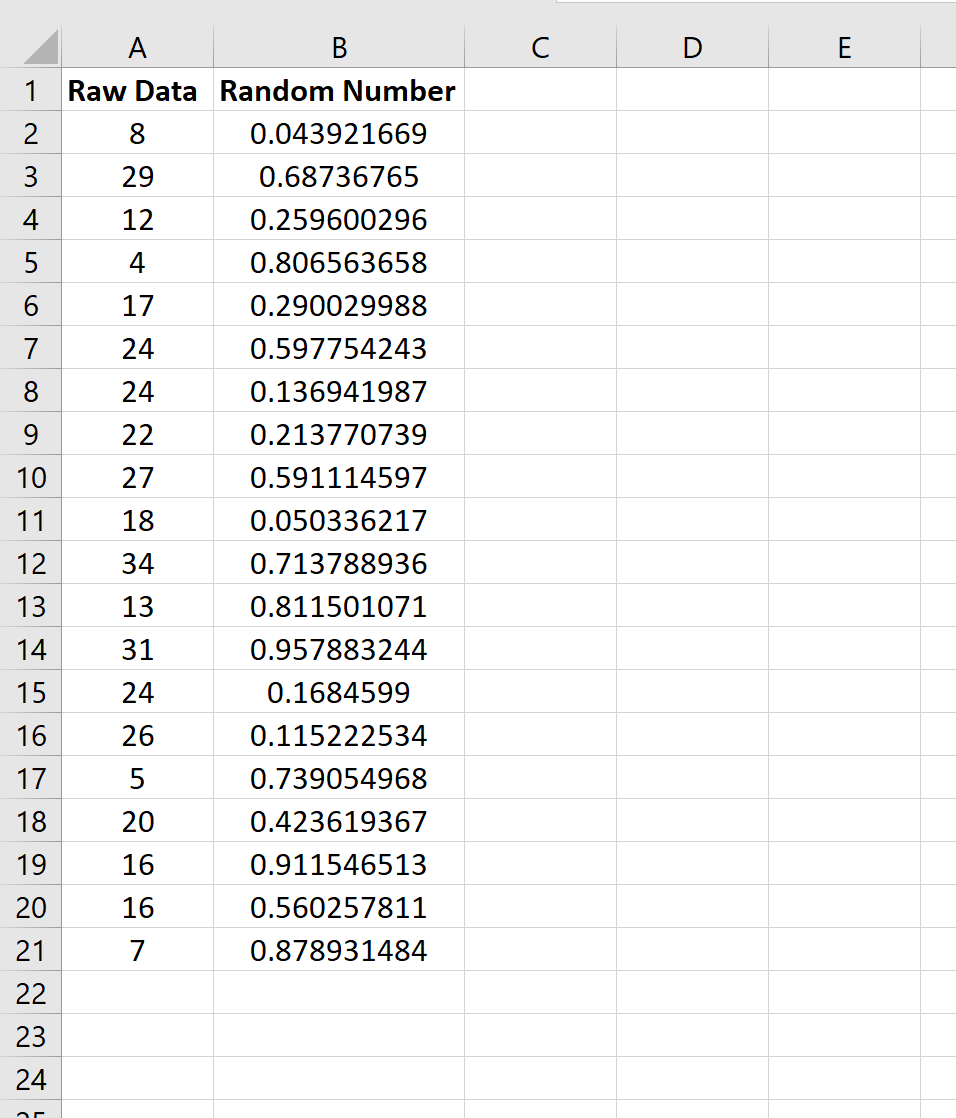
Lastly, highlight the values in column C and drag them to replace the values in column B.
A popup box will appear that says “There’s already data here. Do you want to replace it?” Click OK.
Step 4: Sort by the Random Values
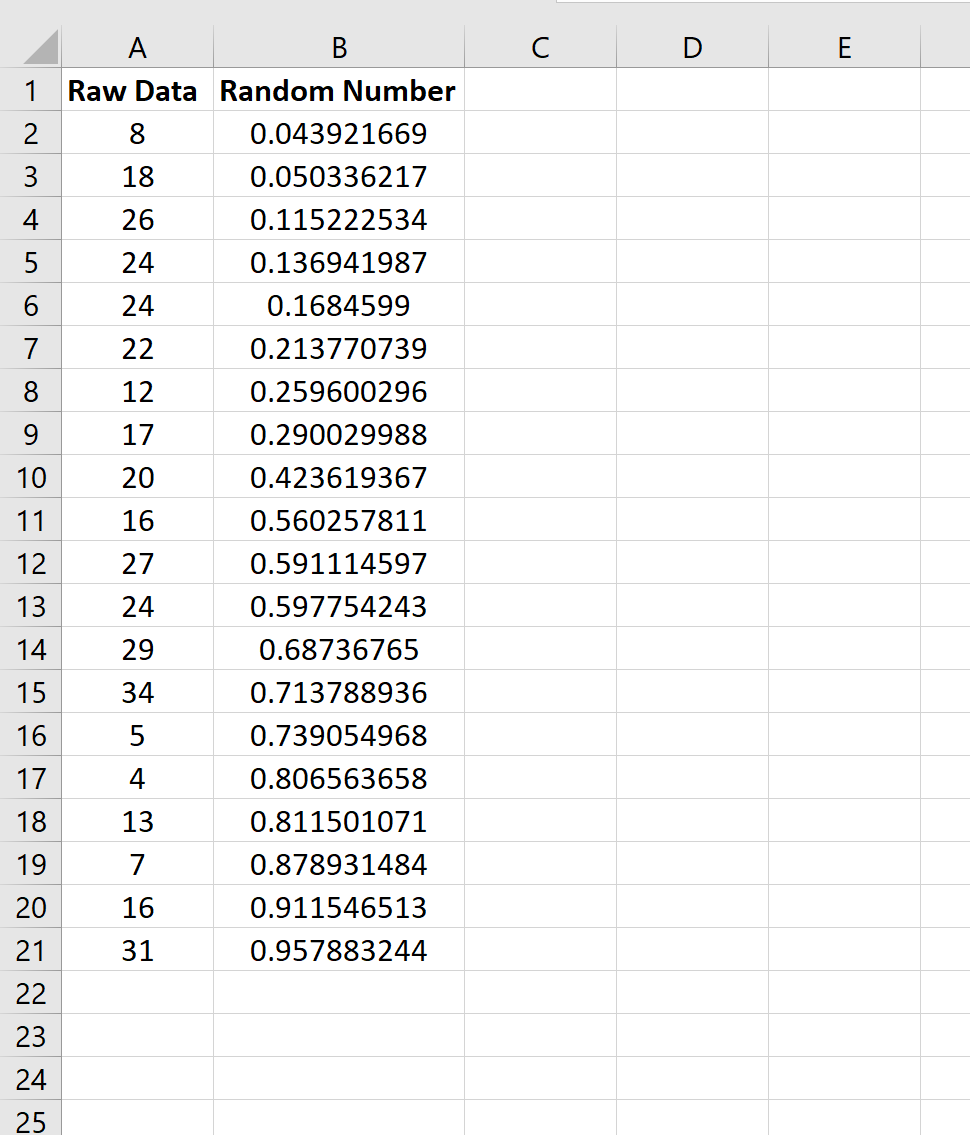
Next, highlight cells A1:B21. Then click the Data tab along the top ribbon, then click Sort within the Sort & Filter section. Sort the values by Random Number smallest to largest.
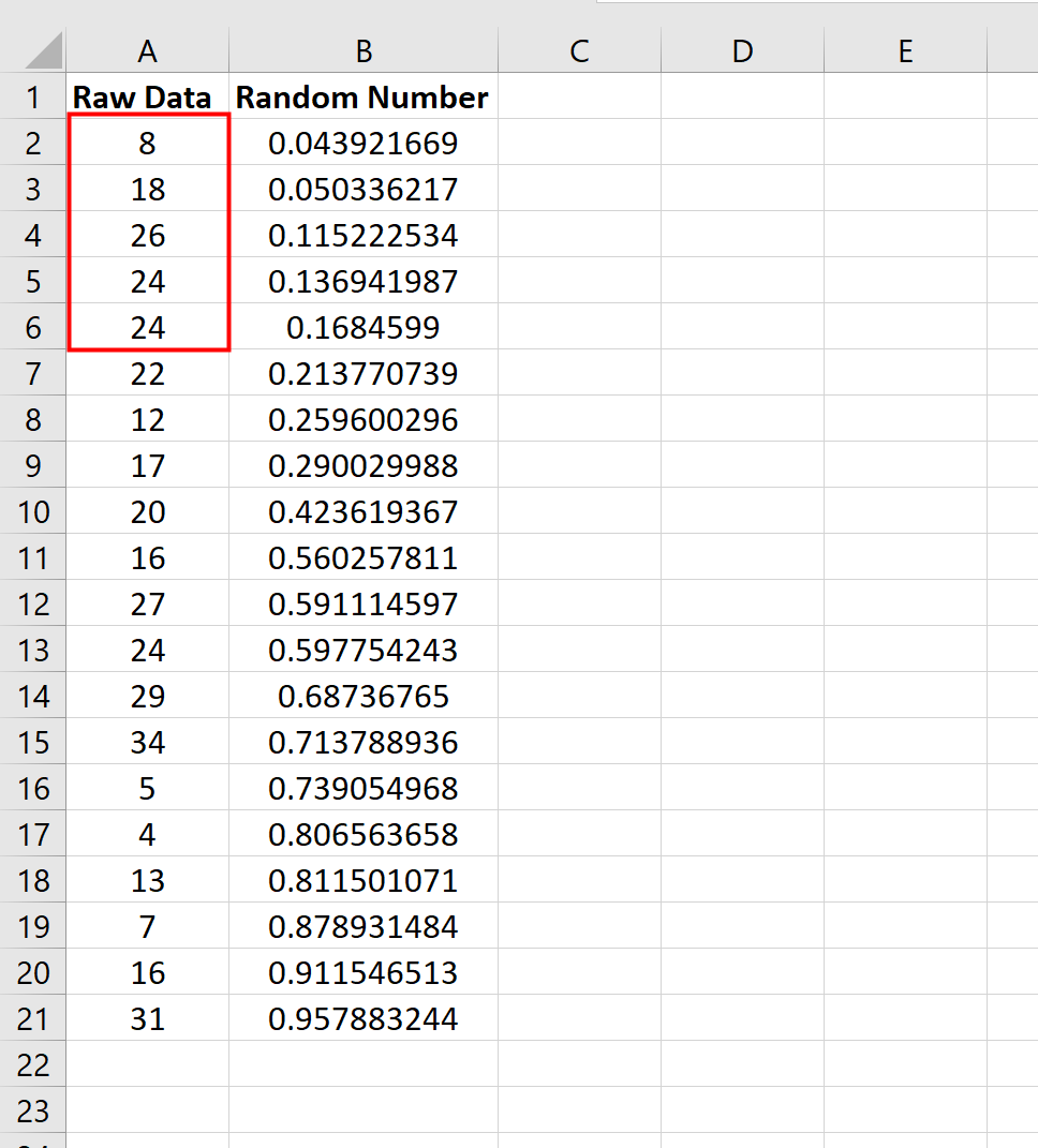
The values will be sorted based on the random number, from smallest to largest:
Step 5: Select the Random Sample
Lastly, choose the first n rows to be in your random sample. For example, if you want a random sample of size 5, then choose the first 5 raw data values to be included in your sample.
In this example, our random sample would include the first 5 values: 8, 18, 26, 24, 24.
