The Pearson correlation coefficient (also known as the “product-moment correlation coefficient”) is a measure of the linear association between two variables X and Y. It has a value between -1 and 1 where:
- -1 indicates a perfectly negative linear correlation between two variables
- 0 indicates no linear correlation between two variables
- 1 indicates a perfectly positive linear correlation between two variables
The Formula to Find the Pearson Correlation Coefficient
The formula to find the Pearson correlation coefficient, denoted as r, for a sample of data is (via Wikipedia):
You will likely never have to compute this formula by hand since you can use software to do this for you, but it’s helpful to have an understanding of what exactly this formula is doing by walking through an example.
Suppose we have the following dataset:

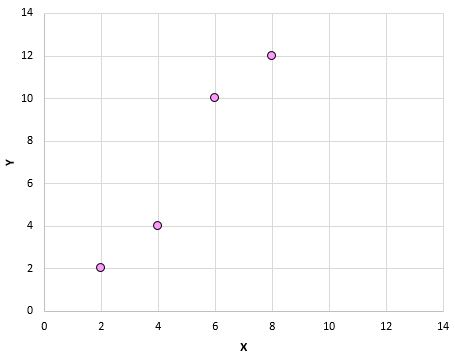
If we plotted these (X, Y) pairs on a scatterplot, it would look like this:
Just from looking at this scatterplot we can tell that there is a positive association between variables X and Y: when X increases, Y tends to increase as well. But to quantify exactly how positively associated these two variables are, we need to find the Pearson correlation coefficient.
Let’s focus on just the numerator of the formula:
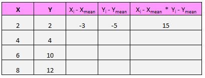
For each (X, Y) pair in our dataset, we need to find the difference between the x value and the mean x value, the difference between the y value and the mean y value, then multiply these two numbers together.
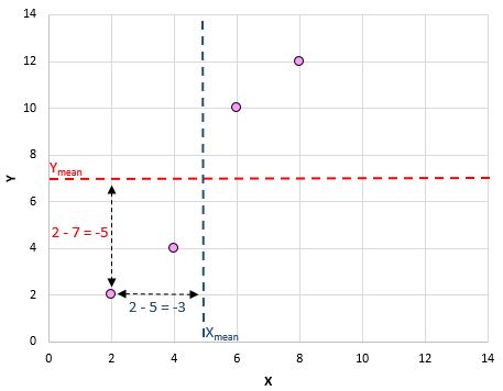
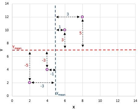
For example, our first (X, Y) pair is (2, 2). The mean x value in this dataset is 5 and the mean y value in this dataset is 7. So, the difference between the x value in this pair and the mean x value is 2 – 5 = -3. The difference between the y value in this pair and the mean y value is 2 – 7 = -5. Then, when we multiply these two numbers together we get -3 * -5 = 15.
Here’s a visual look at what we just did:
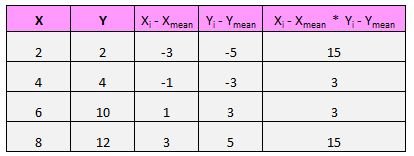
Next, we just need to do this for every single pair:
The last step to get the numerator of the formula is to simply add up all of these values:
15 + 3 +3 + 15 = 36
Next, the denominator of the formula tells us to find the sum of all the squared differences for both x and y, then multiply these two numbers together, then take the square root:
So, first we’ll find the sum of the squared differences for both x and y:
Then we’ll multiply these two numbers together: 20 * 68 = 1,360.
Lastly, we’ll take the square root: √1,360 = 36.88
So, we found the numerator of the formula to be 36 and the denominator to be 36.88. This means that our Pearson correlation coefficient is r = 36 / 36.88 = 0.976
This number is close to 1, which indicates that there is a strong positive linear relationship between our variables X and Y. This confirms the relationship that we saw in the scatterplot.
Visualizing Correlations
Recall that a Pearson correlation coefficient tells us the type of linear relationship (positive, negative, none) between two variables as well as the strength of that relationship (weak, moderate, strong).
When we make a scatterplot of two variables, we can see the actual relationship between two variables. Here are the many different types of linear relationships we might see:
Strong, positive relationship: As the variable on the x-axis increases, the variable on the y-axis increases as well. The dots are packed together tightly, which indicates a strong relationship.
Pearson correlation coefficient: 0.94
Weak, positive relationship: As the variable on the x-axis increases, the variable on the y-axis increases as well. The dots are fairly spread out, which indicates a weak relationship.
Pearson correlation coefficient: 0.44
No relationship: There is no clear relationship (positive or negative) between the variables.
Pearson correlation coefficient: 0.03
Strong, negative relationship: As the variable on the x-axis increases, the variable on the y-axis decreases. The dots are packed tightly together, which indicates a strong relationship.
Pearson correlation coefficient: -0.87
Weak, negative relationship: As the variable on the x-axis increases, the variable on the y-axis decreases. The dots are fairly spread out, which indicates a weak relationship.
Pearson correlation coefficient: –0.46
Testing for Significance of a Pearson Correlation Coefficient
When we find the Pearson correlation coefficient for a set of data, we’re often working with a sample of data that comes from a larger population. This means that it’s possible to find a non-zero correlation for two variables even if they’re actually not correlated in the overall population.
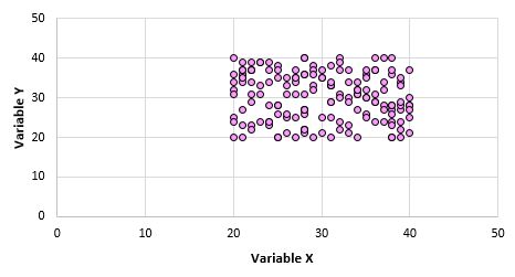
For example, suppose we make a scatterplot for variables X and Y for every data point in the entire population and it looks like this:
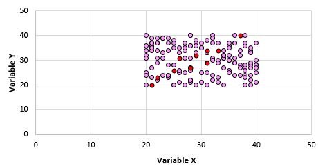
Clearly these two variables are not correlated. However, it’s possible that when we take a sample of 10 points from the population, we choose the following points:
We may find that the Pearson correlation coefficient for this sample of points is 0.93, which indicates a strong positive correlation despite the population correlation being zero.
In order to test for whether or not a correlation between two variables is statistically significant, we can find the following test statistic:
Test statistic T = r * √(n-2) / (1-r2)
where n is the number of pairs in our sample, r is the Pearson correlation coefficient, and test statistic T follows a t distribution with n-2 degrees of freedom.
Let’s walk through an example of how to test for the significance of a Pearson correlation coefficient.
Example
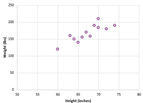
The following dataset shows the height and weight of 12 individuals:

The scatterplot below shows the value of these two variables:
The Pearson correlation coefficient for these two variables is r = 0.836.
The test statistic T = .836 * √(12-2) / (1-.8362) = 4.804.
According to our t distribution calculator, a t score of 4.804 with 10 degrees of freedom has a p-value of .0007. Since .0007
Cautions
While a Pearson correlation coefficient can be useful in telling us whether or not two variables have a linear association, we must keep three things in mind when interpreting a Pearson correlation coefficient:
1. Correlation does not imply causation. Just because two variables are correlated does not mean that one is necessarily causing the other to occur more or less often. A classic example of this is the positive correlation between ice cream sales and shark attacks. When ice cream sales increase during certain times of the year, shark attacks also tend to increase.
Does this mean ice cream consumption is causing shark attacks? Of course not! It just means that during the summer, both ice cream consumption and shark attacks tend to increase since ice cream is more popular during the summer and more people go in the ocean during the summer.
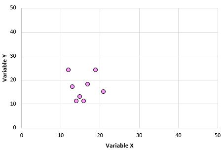
2. Correlations are sensitive to outliers. One extreme outlier can dramatically change a Pearson correlation coefficient. Consider the example below:
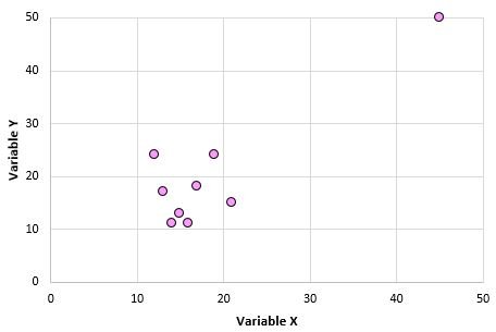
Variables X and Y have a Pearson correlation coefficient of 0.00. But imagine that we have one outlier in the dataset:
Now the Pearson correlation coefficient for these two variables is 0.878. This one outlier changes everything. This is why, when you calculate the correlation for two variables, it’s a good idea to visualize the variables using a scatterplot to check for outliers.
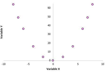
3. A Pearson correlation coefficient does not capture nonlinear relationships between two variables. Imagine that we have two variables with the following relationship:
The Pearson correlation coefficient for these two variables is 0.00 because they have no linear relationship. However, these two variables do have a nonlinear relationship: The y values are simply the x values squared.
When using the Pearson correlation coefficient, keep in mind that you’re merely testing to see if two variables are linearly related. Even if a Pearson correlation coefficient tells us that two variables are uncorrelated, they could still have some type of nonlinear relationship. This is another reason that it’s helpful to create a scatterplot when analyzing the relationship between two variables – it may help you detect a nonlinear relationship.
