A one-way ANOVA is used to determine whether or not different levels of an explanatory variable lead to statistically different results in some response variable.
For example, we might be interested in understanding whether or not three levels of education (Associate’s degree, Bachelor’s degree, Master’s degree) lead to statistically different annual incomes. In this case, we have one explanatory variable and one response variable.
- Explanatory variable: level of education
- Response variable: annual income
A MANOVA is an extension of the one-way ANOVA in which there is more than one response variable. For example, we might be interested in understanding whether or not level of education leads to different annual incomes and different amounts of student loan debt. In this case, we have one explanatory variable and two response variables:
- Explanatory variable: level of education
- Response variables: annual income, student loan debt
Because we have more than one response variable, it would be appropriate to use a MANOVA in this case.
In this tutorial, we’ll explain how to perform a MANOVA in SPSS.
Example: MANOVA in SPSS
To illustrate how to perform a MANOVA in SPSS, we’ll use the following dataset that contains the following three variables for 24 individuals:
- educ: level of education (0 = Associate, 1 = Bachelor, 2 = Master)
- income: annual income
- debt: total student loan debt

Use the following steps to perform a MANOVA in SPSS:
Step 1: Perform a MANOVA.
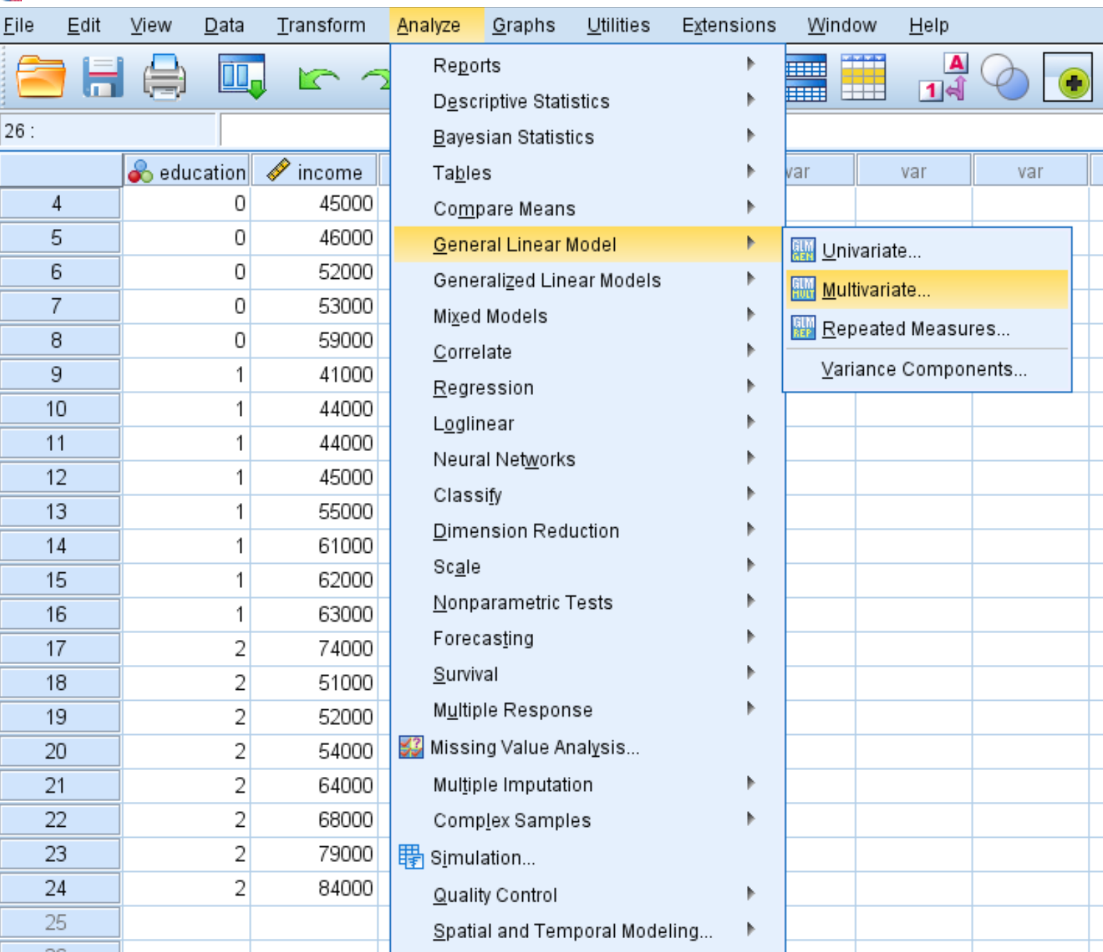
Click the Analyze tab, then General Linear Model, then Multivariate:
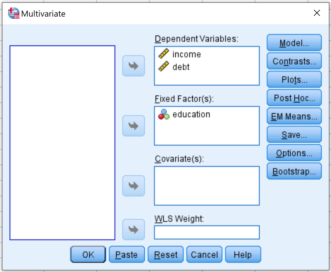
In the new window that pops up, drag the variables income and debt into the box labelled Dependent Variables. Then drag the factor variable education into the box labelled Fixed Factors:
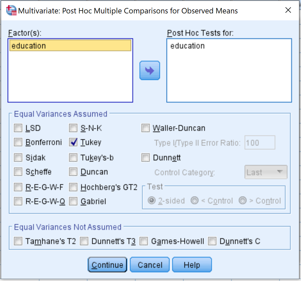
Next, click the button Post Hoc. Drag the factor education into the box labelled Post Hoc Tests for. Then check the box next to Tukey. Then click Continue.
Lastly, click OK.
Step 2: Interpret the results.
Once you click OK, the results of the MANOVA will appear. Here is how to interpret the output:
Multivariate Tests
This table tells you whether or not level of education leads to statistically significant differences in annual income and total student debt. We will look at the numbers in the row titled Wilks’ Lambda:
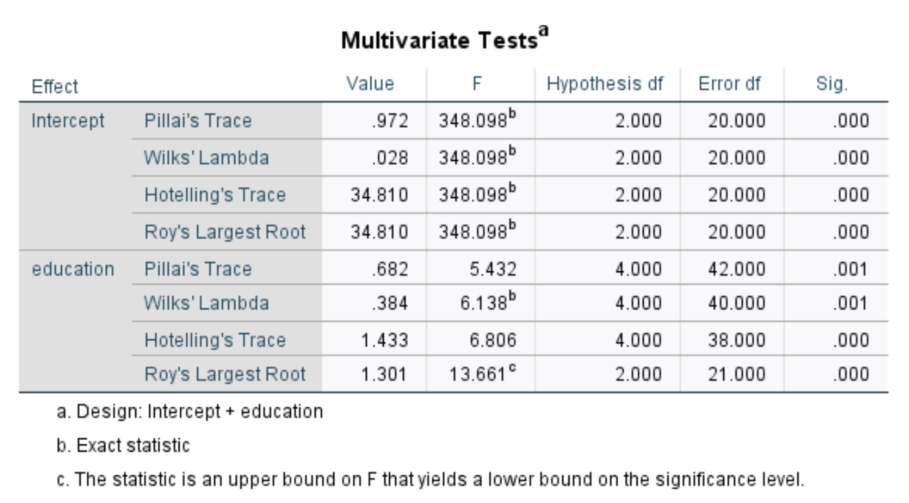
The overall F statistic is 6.138 and the corresponding p-value is .001. Since this value is less than .05, this indicates that level of education does have a significant effect on annual income and total student debt.
Tests of Between-Subjects Effects
This table shows the individual p-values for both income and debt:
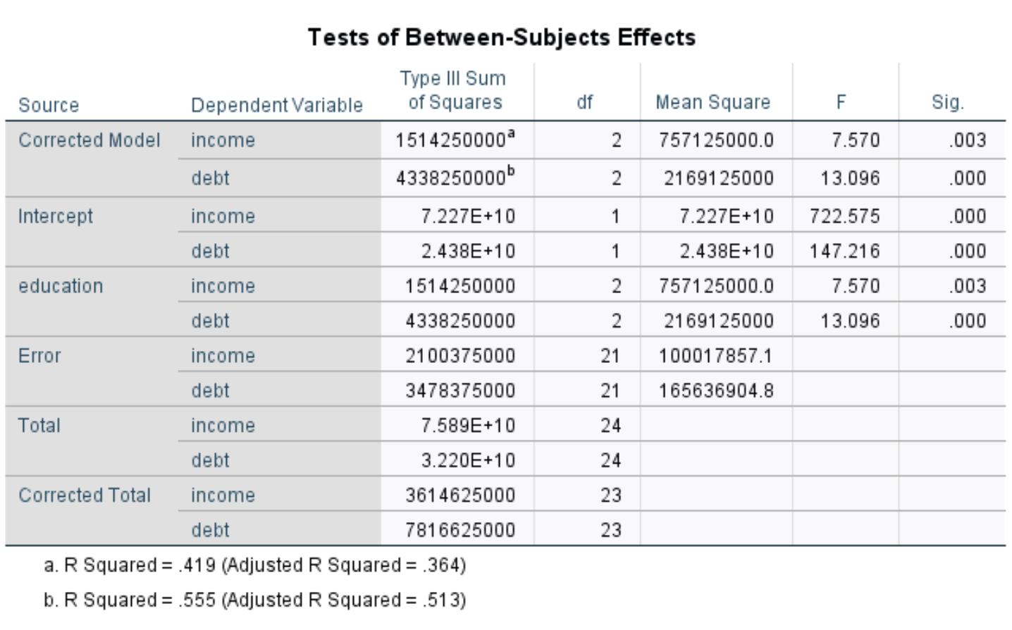
The p-value for income is .003 and the p-value for debt is .000. Since both of these values are less than .05, it means that level of education has a statistically significant effect on both income and debt.
Post Hoc Tests
This table displays the Tukey post hoc comparisons for each level of education.
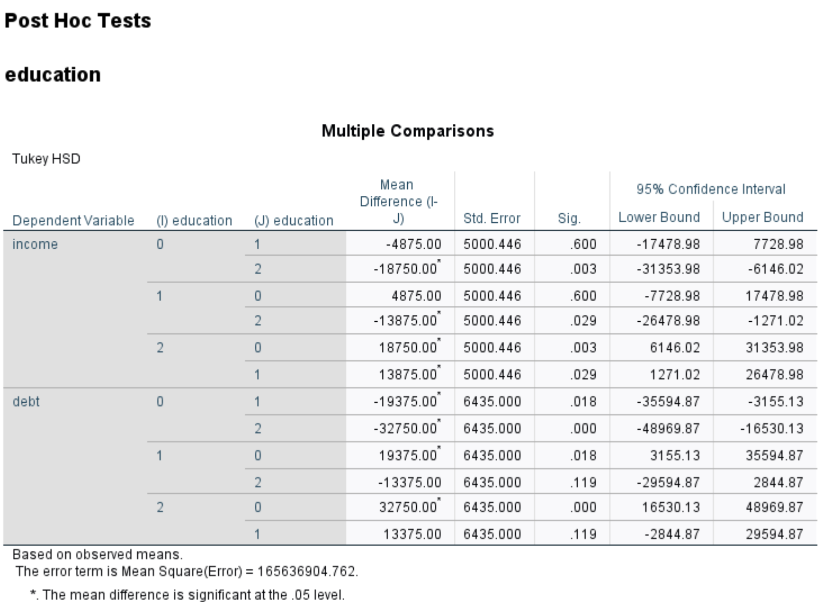
From the table we can observe the following:
- The amount of income for individuals with an Associate’s degree (education=0) is significantly different than the amount of income for individuals with a Master’s degree (education=1) | p-value = .003.
- The amount of income for individuals with a Bachelor’s degree (education=1) is significantly different than the amount of income for individuals with a Master’s degree (education=2) | p-value = .029.
- The amount of income for individuals with an Associate’s degree (education=0) is significantly different than the amount of income for individuals with a Bachelor’s degree (education=1) | p-value = .018.
- The amount of income for individuals with an Associate’s degree (education=0) is significantly different than the amount of income for individuals with a Master’s degree (education=2) | p-value = .000.
Further Reading: The Differences Between ANOVA, ANCOVA, MANOVA, and MANCOVA