How to Perform Logistic Regression in R (Step-by-Step)

---

Logistic regression is a method we can use to fit a regression model when the response variable is binary.

Logistic regression uses a method known as maximum likelihood estimation to find an equation of the following form:

log[p(X) / (1-p(X))]  =  β₀ + β₁X₁ + β₂X₂ + … + β_pX_p

where:

• X_j: The j^th predictor variable
• β_j: The coefficient estimate for the j^th predictor variable

The formula on the right side of the equation predicts the log odds of the response variable taking on a value of 1.

Thus, when we fit a logistic regression model we can use the following equation to calculate the probability that a given observation takes on a value of 1:

p(X) = e^{β₀ + β₁X₁ + β₂X₂ + … + β_pX_p} / (1 + e^{β₀ + β₁X₁ + β₂X₂ + … + β_pX_p})

We then use some probability threshold to classify the observation as either 1 or 0.

For example, we might say that observations with a probability greater than or equal to 0.5 will be classified as “1” and all other observations will be classified as “0.”

This tutorial provides a step-by-step example of how to perform logistic regression in R.

Step 1: Load the Data

For this example, we’ll use the Default dataset from the ISLR package. We can use the following code to load and view a summary of the dataset:

#load dataset
data #view summary of dataset
summary(data)

 default    student       balance           income     
 No :9667   No :7056   Min.   :   0.0   Min.   :  772  
 Yes: 333   Yes:2944   1st Qu.: 481.7   1st Qu.:21340  
                       Median : 823.6   Median :34553  
                       Mean   : 835.4   Mean   :33517  
                       3rd Qu.:1166.3   3rd Qu.:43808  
                       Max.   :2654.3   Max.   :73554  

#find total observations in dataset
nrow(data)

[1] 10000

This dataset contains the following information about 10,000 individuals:

• default: Indicates whether or not an individual defaulted.
• student: Indicates whether or not an individual is a student.
• balance: Average balance carried by an individual.
• income: Income of the individual.

We will use student status, bank balance, and income to build a logistic regression model that predicts the probability that a given individual defaults.

Step 2: Create Training and Test Samples

Next, we’ll split the dataset into a training set to train the model on and a testing set to test the model on.

#make this example reproducible
set.seed(1)

#Use 70% of dataset as training set and remaining 30% as testing set
sample TRUE, FALSE), nrow(data), replace=TRUE, prob=c(0.7,0.3))
train 

Step 3: Fit the Logistic Regression Model

Next, we’ll use the glm (general linear model) function and specify family=”binomial” so that R fits a logistic regression model to the dataset:

#fit logistic regression model
model binomial", data=train)

#disable scientific notation for model summary
options(scipen=999)

#view model summary
summary(model)

Call:
glm(formula = default ~ student + balance + income, family = "binomial", 
    data = train)

Deviance Residuals: 
    Min       1Q   Median       3Q      Max  
-2.5586  -0.1353  -0.0519  -0.0177   3.7973  

Coefficients:
                 Estimate    Std. Error z value            Pr(>|z|)    
(Intercept) -11.478101194   0.623409555 -18.412 

The coefficients in the output indicate the average change in log odds of defaulting. For example, a one unit increase in balance is associated with an average increase of 0.005988 in the log odds of defaulting.

The p-values in the output also give us an idea of how effective each predictor variable is at predicting the probability of default:

• P-value of student status: 0.0843
• P-value of balance: 
• P-value of income: 0.4304

We can see that balance and student status seem to be important predictors since they have low p-values while income is not nearly as important.

Assessing Model Fit:

In typical linear regression, we use R² as a way to assess how well a model fits the data. This number ranges from 0 to 1, with higher values indicating better model fit.

However, there is no such R² value for logistic regression. Instead, we can compute a metric known as McFadden’s R², which ranges from 0 to just under 1. Values close to 0 indicate that the model has no predictive power. In practice, values over 0.40 indicate that a model fits the data very well.

We can compute McFadden’s R² for our model using the pR2 function from the pscl package:

pscl::pR2(model)["McFadden"]

 McFadden 
0.4728807 

A value of 0.4728807 is quite high for McFadden’s R², which indicates that our model fits the data very well and has high predictive power.

Variable Importance:

We can also compute the importance of each predictor variable in the model by using the varImp function from the caret package:

caret::varImp(model)

             Overall
studentYes  1.726393
balance    20.383812
income      0.788449

Higher values indicate more importance. These results match up nicely with the p-values from the model. Balance is by far the most important predictor variable, followed by student status and then income.

VIF Values:

We can also calculate the VIF values of each variable in the model to see if multicollinearity is a problem:

#calculate VIF values for each predictor variable in our model
car::vif(model)

 student  balance   income 
2.754926 1.073785 2.694039

As a rule of thumb, VIF values above 5 indicate severe multicollinearity. Since none of the  predictor variables in our models have a VIF over 5, we can assume that multicollinearity is not an issue in our model.

Step 4: Use the Model to Make Predictions

Once we’ve fit the logistic regression model, we can then use it to make predictions about whether or not an individual will default based on their student status, balance, and income:

#define two individuals
new Yes", "No"))

#predict probability of defaulting
predict(model, new, type="response")

         1          2 
0.02732106 0.04397747

The probability of an individual with a balance of $1,400, an income of $2,000, and a student status of “Yes” has a probability of defaulting of .0273. Conversely, an individual with the same balance and income but with a student status of “No” has a probability of defaulting of 0.0439. 

We can use the following code to calculate the probability of default for every individual in our test dataset:

#calculate probability of default for each individual in test dataset
predicted response")

Step 5: Model Diagnostics

Lastly, we can analyze how well our model performs on the test dataset.

By default, any individual in the test dataset with a probability of default greater than 0.5 will be predicted to default. However, we can find the optimal probability to use to maximize the accuracy of our model by using the optimalCutoff() function from the InformationValue package:

library(InformationValue)

#convert defaults from "Yes" and "No" to 1's and 0's
test$default ifelse(test$default=="Yes", 1, 0)

#find optimal cutoff probability to use to maximize accuracy
optimal 

This tells us that the optimal probability cutoff to use is 0.5451712. Thus, any individual with a probability of defaulting of 0.5451712 or higher will be predicted to default, while any individual with a probability less than this number will be predicted to not default.

Using this threshold, we can create a confusion matrix which shows our predictions compared to the actual defaults:

confusionMatrix(test$default, predicted)

     0  1
0 2912 64
1   21 39

We can also calculate the sensitivity (also known as the “true positive rate”) and specificity (also known as the “true negative rate”) along with the total misclassification error (which tells us the percentage of total incorrect classifications):

#calculate sensitivity
sensitivity(test$default, predicted)

[1] 0.3786408

#calculate specificity
specificity(test$default, predicted)

[1] 0.9928401

#calculate total misclassification error rate
misClassError(test$default, predicted, threshold=optimal)

[1] 0.027

The total misclassification error rate is 2.7% for this model. In general, the lower this rate the better the model is able to predict outcomes, so this particular model turns out to be very good at predicting whether an individual will default or not.

Lastly, we can plot the ROC (Receiver Operating Characteristic) Curve which displays the percentage of true positives predicted by the model as the prediction probability cutoff is lowered from 1 to 0. The higher the AUC (area under the curve), the more accurately our model is able to predict outcomes:

#plot the ROC curve
plotROC(test$default, predicted)

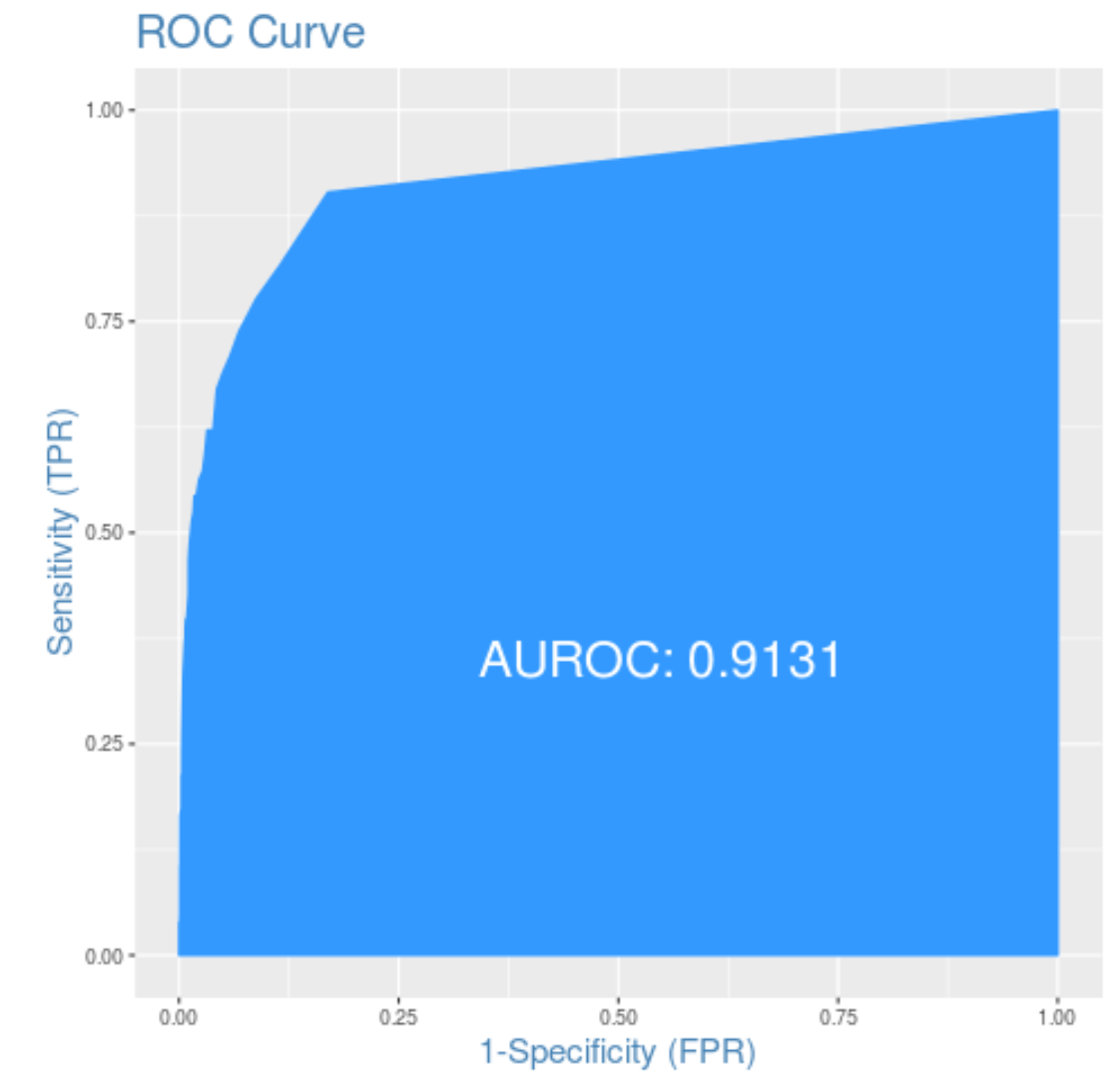
We can see that the AUC is 0.9131, which is quite high. This indicates that our model does a good job of predicting whether or not an individual will default.