Multiple linear regression is one of the most commonly used techniques in all of statistics.
This tutorial explains how to interpret every value in the output of a multiple linear regression model in Excel.
Example: Interpreting Regression Output in Excel
Suppose we want to know if the number of hours spent studying and the number of prep exams taken affects the score that a student receives on a certain college entrance exam.
To explore this relationship, we can perform multiple linear regression using hours studied and prep exams taken as predictor variables and exam score as a response variable.
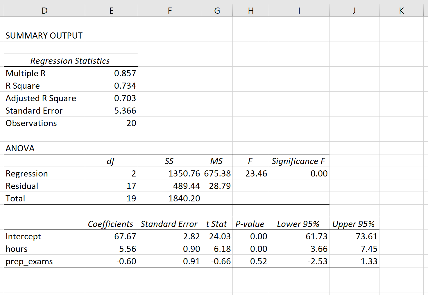
The following screenshot shows the regression output of this model in Excel:

Here is how to interpret the most important values in the output:
Multiple R: 0.857. This represents the multiple correlation between the response variable and the two predictor variables.
R Square: 0.734. This is known as the coefficient of determination. It is the proportion of the variance in the response variable that can be explained by the explanatory variables. In this example, 73.4% of the variation in the exam scores can be explained by the number of hours studied and the number of prep exams taken.
Adjusted R Square: 0.703. This represents the R Square value, adjusted for the number of predictor variables in the model. This value will also be less than the value for R Square and penalizes models that use too many predictor variables in the model.
Standard error: 5.366. This is the average distance that the observed values fall from the regression line. In this example, the observed values fall an average of 5.366 units from the regression line.
Observations: 20. The total sample size of the dataset used to produce the regression model.
F: 23.46. This is the overall F statistic for the regression model, calculated as regression MS / residual MS.
Significance F: 0.0000. This is the p-value associated with the overall F statistic. It tells us whether or not the regression model as a whole is statistically significant.
In this case the p-value is less than 0.05, which indicates that the explanatory variables hours studied and prep exams taken combined have a statistically significant association with exam score.
Coefficients: The coefficients for each explanatory variable tell us the average expected change in the response variable, assuming the other explanatory variable remains constant.
For example, for each additional hour spent studying, the average exam score is expected to increase by 5.56, assuming that prep exams taken remains constant.
We interpret the coefficient for the intercept to mean that the expected exam score for a student who studies zero hours and takes zero prep exams is 67.67.
P-values. The individual p-values tell us whether or not each explanatory variable is statistically significant. We can see that hours studied is statistically significant (p = 0.00) while prep exams taken (p = 0.52) is not statistically significant at α = 0.05.
How to Write the Estimated Regression Equation
We can use the coefficients from the output of the model to create the following estimated regression equation:
Exam score = 67.67 + 5.56*(hours) – 0.60*(prep exams)
We can use this estimated regression equation to calculate the expected exam score for a student, based on the number of hours they study and the number of prep exams they take.
For example, a student who studies for three hours and takes one prep exam is expected to receive a score of 83.75:
Exam score = 67.67 + 5.56*(3) – 0.60*(1) = 83.75
Keep in mind that because prep exams taken was not statistically significant (p = 0.52), we may decide to remove it because it doesn’t add any improvement to the overall model.
In this case, we could perform simple linear regression using only hours studied as the explanatory variable.
Additional Resources
Introduction to Simple Linear Regression
Introduction to Multiple Linear Regression