You can use the following formula with IFERROR and VLOOKUP in Google Sheets to return a value other than #N/A when the VLOOKUP function does not find a particular value in a range:
=IFERROR(VLOOKUP("string",A2:B11,2,FALSE),"Does Not Exist")
This particular formula looks for “string” in the range A2:B11 and attempts to return the corresponding value in the second column of this range.
If it does not find “string” then it simply returns “Does Not Exist” instead of a #N/A value.
The following example shows how to use this formula in practice.
Example: Use IFERROR with VLOOKUP in Google Sheets
Suppose we have the following dataset that shows the number of points scored by various basketball teams:

Suppose we use the following VLOOKUP formula to find the number of points associated with the “Raptors” team:
=VLOOKUP("Raptors",A2:B11,2,FALSE)
The following screenshot shows how to use this formula:

This formula returns a value of #N/A because the “Raptors” do not exist in the Team column.
However, we can use the following IFERROR function with the VLOOKUP function to return a value of “Does Not Exist” instead of #N/A:
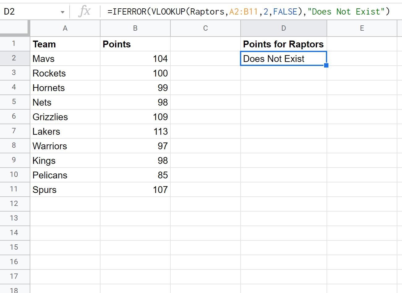
=IFERROR(VLOOKUP("Raptors",A2:B11,2,FALSE),"Does Not Exist")
The following screenshot shows how to use this formula:

Since the “Raptors” do not exist in the Team column, the formula returns a value of “Does Not Exist” instead of a #N/A value.
Additional Resources
The following tutorials explain how to perform other common operations in Google Sheets:
How to Use a Case Sensitive VLOOKUP in Google Sheets
How to Use a Case Sensitive VLOOKUP in Google Sheets