You can use the following syntax to use a VLOOKUP by date in Google Sheets:
=VLOOKUP(D2, A2:B9, 2, FALSE)
This particular formula looks up the date in cell D2 in the range A2:B9 and returns the corresponding value in column 2 of the range.
Note: The FALSE argument tells Google Sheets to look for exact matches instead of approximate matches.
The following example shows how to use this syntax in practice.
Example: Use VLOOKUP by Date in Google Sheets
Suppose we have the following dataset in Google Sheets that shows the total sales of some product on various dates:

We can use the following formula with VLOOKUP to look up the date value in cell D2 in column A and return the corresponding sales value in column B:
=VLOOKUP(D2, A2:B9, 2, FALSE)
The following screenshot shows how to use this formula in practice:
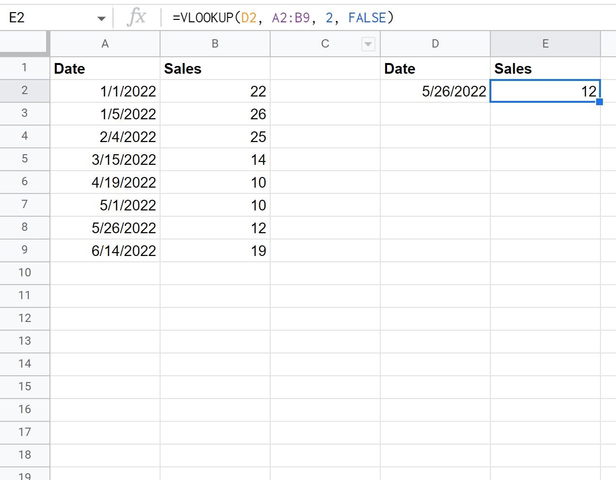
The VLOOKUP formula returns 12, which is the sales value that corresponds to the date 5/26/2022 in the original dataset.
Note that this formula assumes the values in column A are in a valid date format and that the value we supply to the VLOOKUP formula is also in a valid date format.
If the value that we supply to the VLOOKUP formula is not valid, then the formula will simply return #N/A as a result:

Since 5.26.2022 is not a valid date format, the VLOOKUP formula returns #N/A as a result.
Additional Resources
The following tutorials explain how to perform other common tasks in Google Sheets:
Google Sheets: How to Use VLOOKUP From Another Workbook
Google Sheets: Use VLOOKUP to Return All Matches
Google Sheets: Use VLOOKUP with Multiple Criteria