You can use the following basic syntax to reverse a text string in Google Sheets:
=JOIN("",ArrayFormula(MID(A2,LEN(A2)-SEQUENCE(1,LEN(A2))+1,1)))
This particular formula will reverse the text string located in cell A2.
The following example shows how to use this formula in practice.
Example: Reverse a Text String in Google Sheets
Suppose we have the following list of text strings in Google Sheets:

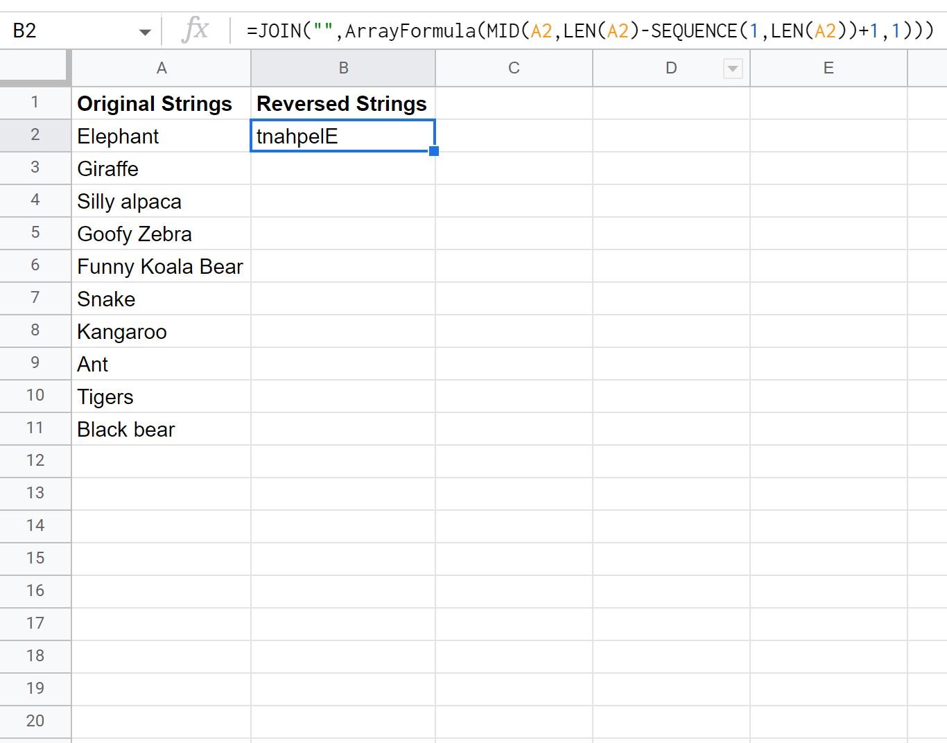
We can type the following formula into cell B2 to reverse the text string in cell A2:
=JOIN("",ArrayFormula(MID(A2,LEN(A2)-SEQUENCE(1,LEN(A2))+1,1)))
The following screenshot shows how to use this formula in practice:

Notice that the first text string of Elephant has been reversed to tnahpelE.
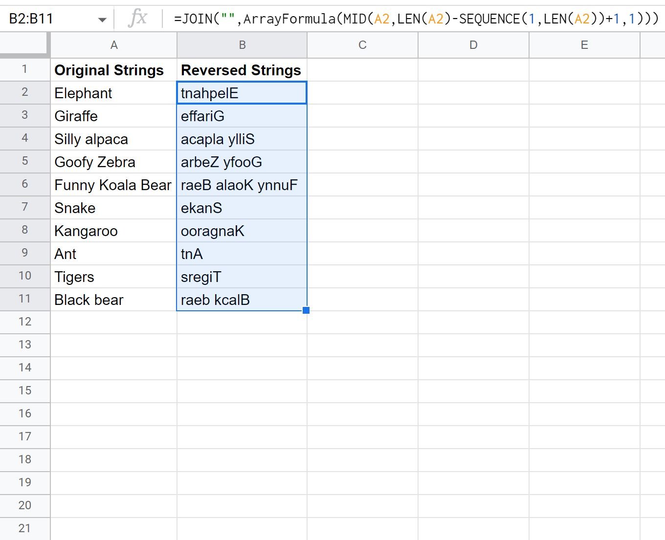
We can then drag and fill this formula down to each remaining cell in column B:

Notice that column B contains the exact reverse of each text string in column A.
Also notice that this formula is able to handle text strings with multiple words and spaces.
Additional Resources
The following tutorials explain how to perform other common tasks in Google Sheets:
Google Sheets: Use VLOOKUP with Multiple Criteria
Google Sheets: How to Perform a Reverse VLOOKUP
Google Sheets: How to Filter with Multiple Conditions