You can use the following basic syntax to calculate different metrics in Google Sheets while ignoring #N/A values:
=AVERAGE(IFNA(A2:A14, ""))

=SUM(IFNA(A2:A14, ""))

=IFNA(VLOOKUP(E2, A2:A14, 2, FALSE), "")
These formulas simply replace #N/A values with blanks and then calculates the metric you’re interested in.
The following examples show how to use this syntax in practice.
Example 1: Calculate Average & Ignore #N/A Values
The following screenshot shows how to calculate the average of a dataset that contains #N/A values:

The average value of the dataset (ignoring all #N/A values) is 9.7.
Example 2: Calculate Sum & Ignore #N/A Values
The following screenshot shows how to calculate the sum of a dataset that contains #N/A values:
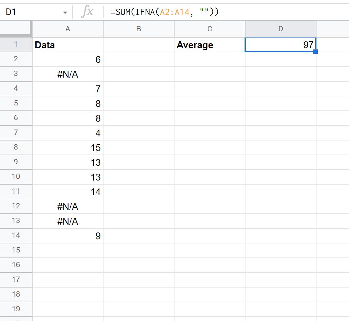
The sum of the dataset (ignoring all #N/A values) is 97.
Example 3: Use VLOOKUP & Ignore #N/A Values
The following screenshot shows how to use the VLOOKUP function to return the value in the Points column that corresponds to the value in the Team column:
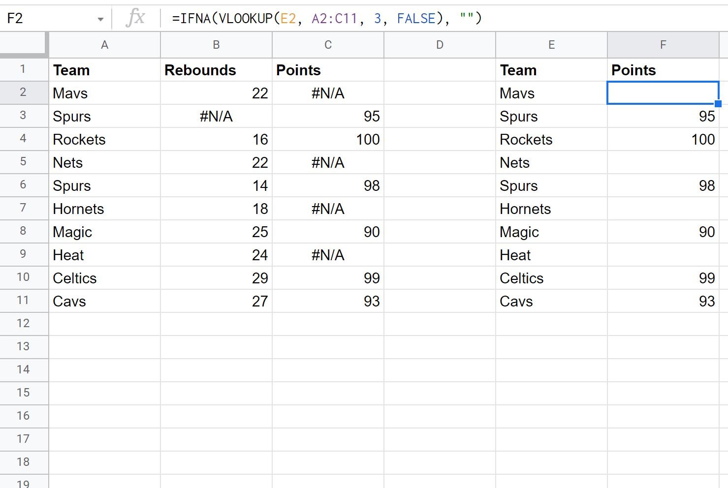
Notice that for any value in the Points column equal to #N/A, the VLOOKUP function simply returns a blank value instead of a #N/A value.
Additional Resources
The following tutorials explain how to perform other common tasks in Google Sheets:
How to Remove Special Characters in Google Sheets
How to Use a Case Sensitive VLOOKUP in Google Sheets
How to Use ISERROR in Google Sheets