By default, the XLOOKUP function in Excel looks up some value in a range and returns a corresponding value only for the first match.
However, you can use the FILTER function instead to look up some value in a range and return corresponding values for all matches:
=FILTER(C2:C11, E2=A2:A11)
This particular formula looks in the range C2:C11 and returns the corresponding values in the range A2:A11 for all rows where the value in C2:C11 is equal to E2.
The following example shows how to use this syntax in practice.
Example: Use XLOOKUP to Return All Matches
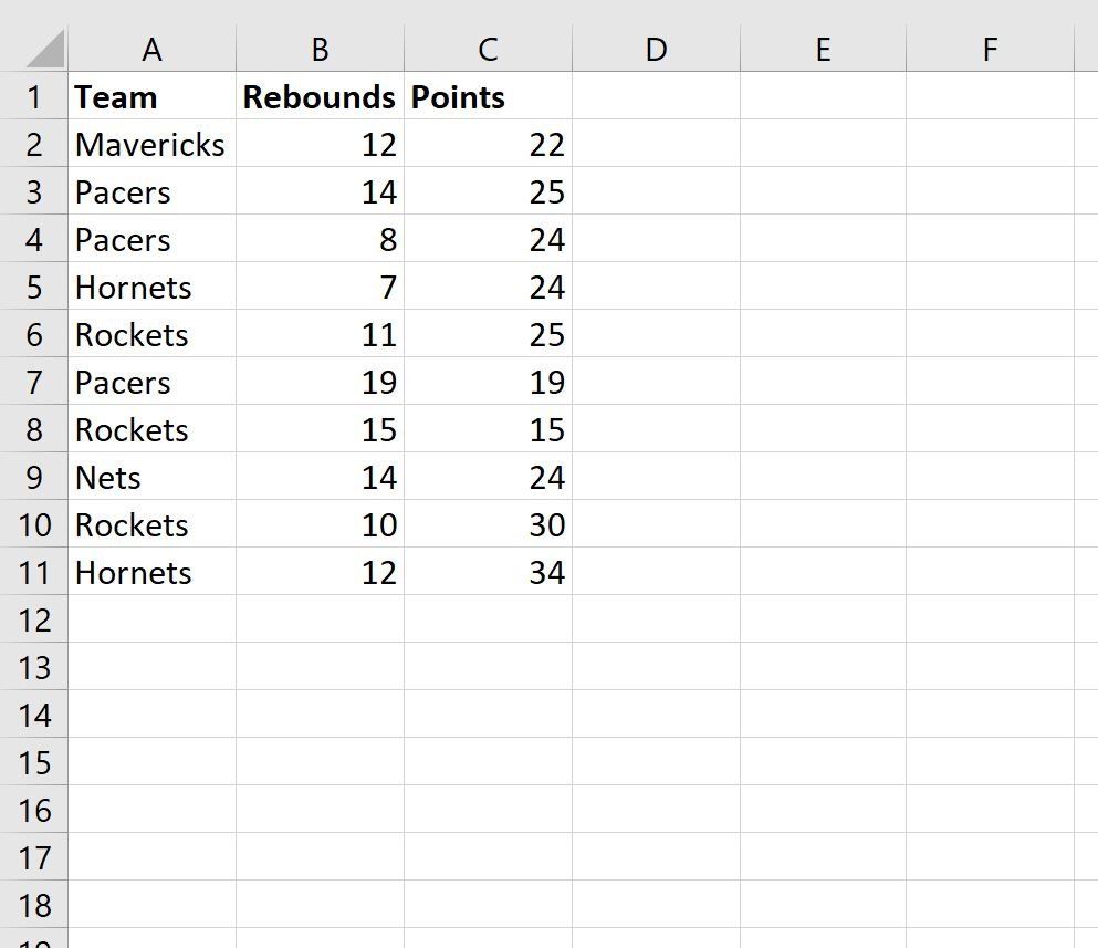
Suppose we have the following dataset in Excel that shows information about various basketball teams:
Suppose we use the following formula with XLOOKUP to look up the team “Rockets” in column A and return the corresponding points value in column C:
=XLOOKUP(E2, A2:A11, C2:C11)
The following screenshot shows how to use this formula in practice:
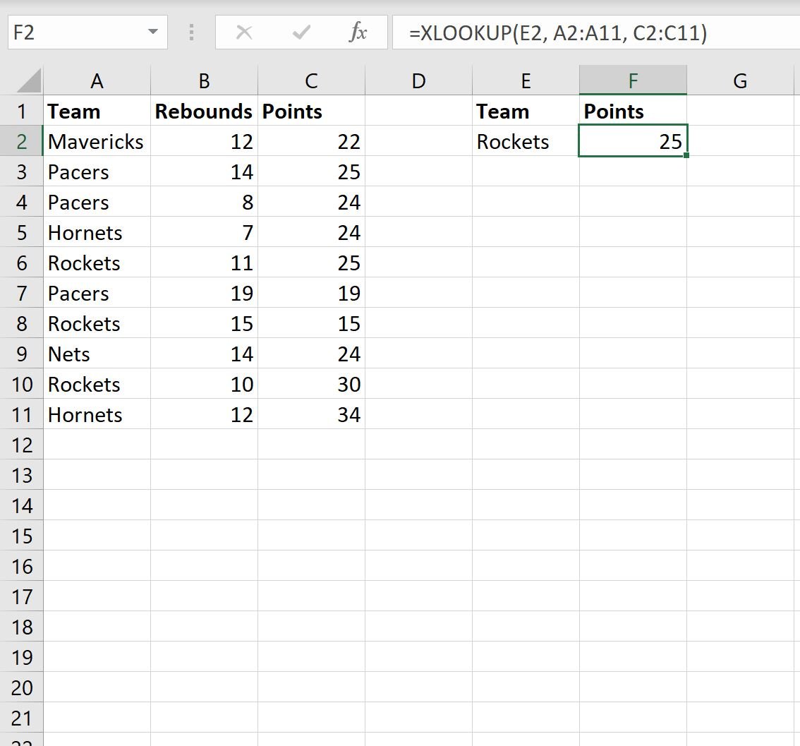
The XLOOKUP function returns the value in the “Points” column for the first occurrence of Rockets in the “Team” column, but it fails to return the points values for the other two rows that also contain Rockets in the “Team” column.
To return the points values for all rows that contain Rockets in the “Team” column, we can use the FILTER function instead.
Here’s the exact formula we can use:
=FILTER(C2:C11, E2=A2:A11)
The following screenshot shows how to use this formula in practice:
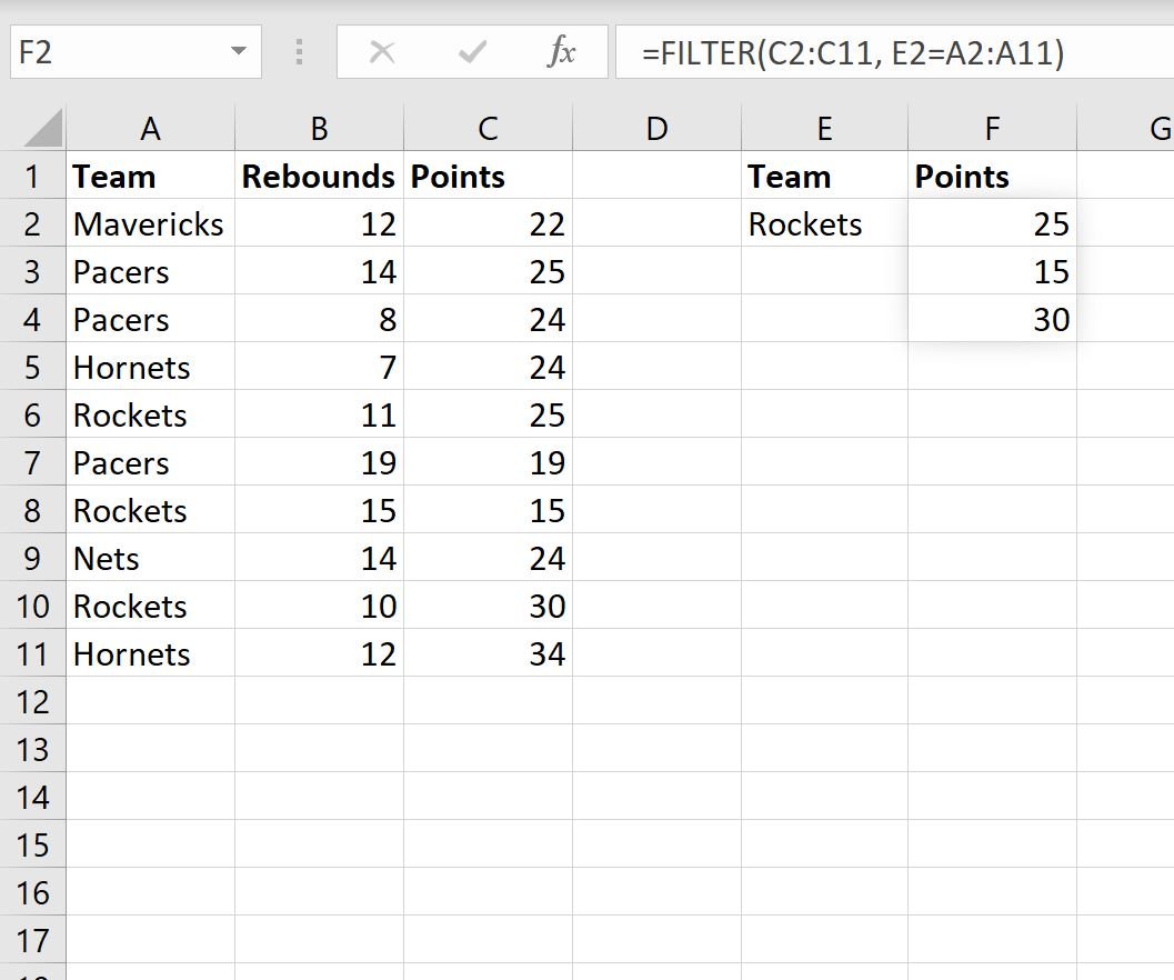
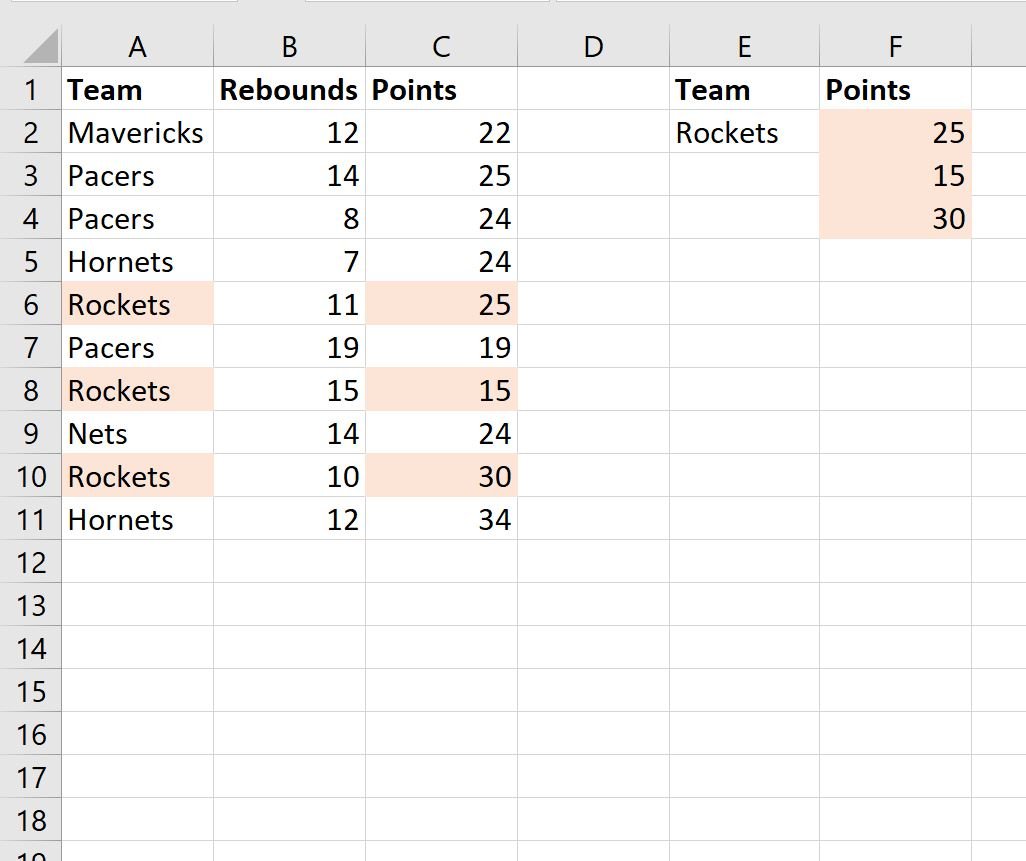
Notice that the FILTER function returns all three points values for the three rows where the “Team” column contains Rockets.
Related: How to Use XLOOKUP with Multiple Criteria in Excel
Additional Resources
The following tutorials explain how to perform other common operations in Excel:
How to Compare Two Lists in Excel Using VLOOKUP
How to Find Unique Values from Multiple Columns in Excel
How to Filter Multiple Columns in Excel