There are two main branches in the field of statistics:
- Descriptive Statistics
- Inferential Statistics
This tutorial explains the difference between the two branches and why each one is useful in certain situations.
Descriptive Statistics
In a nutshell, descriptive statistics aims to describe a chunk of raw data using summary statistics, graphs, and tables.
Descriptive statistics are useful because they allow you to understand a group of data much more quickly and easily compared to just staring at rows and rows of raw data values.
For example, suppose we have a set of raw data that shows the test scores of 1,000 students at a particular school. We might be interested in the average test score along with the distribution of test scores.
Using descriptive statistics, we could find the average score and create a graph that helps us visualize the distribution of scores.
This allows us to understand the test scores of the students much more easily compared to just staring at the raw data.
Common Forms of Descriptive Statistics
There are three common forms of descriptive statistics:
1. Summary statistics. These are statistics that summarize the data using a single number. There are two popular types of summary statistics:
- Measures of central tendency: these numbers describe where the center of a dataset is located. Examples include the mean and the median.
- Measures of dispersion: these numbers describe how spread out the values are in the dataset. Examples include the range, interquartile range, standard deviation, and variance.
2. Graphs. Graphs help us visualize data. Common types of graphs used to visualize data include boxplots, histograms, stem-and-leaf plots, and scatterplots.
3. Tables. Tables can help us understand how data is distributed. One common type of table is a frequency table, which tells us how many data values fall within certain ranges.
Example of Using Descriptive Statistics
The following example illustrates how we might use descriptive statistics in the real world.
Suppose 1,000 students at a certain school all take the same test. We are interested in understanding the distribution of test scores, so we use the following descriptive statistics:
1. Summary Statistics
Mean: 82.13. This tells us that the average test score among all 1,000 students is 82.13.
Median: 84. This tells us that half of all students scored higher than 84 and half scored lower than 84.
Max: 100. Min: 45. This tells us the maximum score that any student obtained was 100 and the minimum score was 45. The range – which tells us the difference between the max and the min – is 55.
2. Graphs
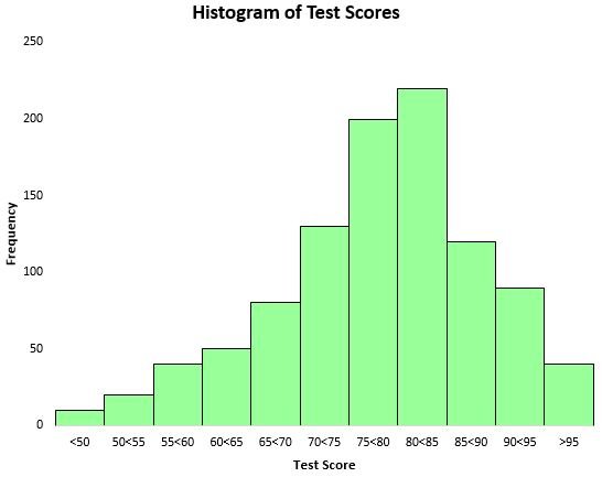
To visualize the distribution of test scores, we can create a histogram – a type of chart that uses rectangular bars to represent frequencies.

Based on this histogram, we can see that the distribution of test scores is roughly bell-shaped. Most of the students scored between 70 and 90, while very few scored above 95 and fewer still scored below 50.
3. Tables
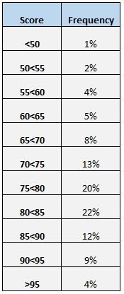
Another easy way to gain an understanding of the distribution of scores is to create a frequency table. For example, the following frequency table shows what percentage of students scored between various ranges:

We can see that just 4% of the total students scored above a 95. We can also see that (12% + 9% + 4% = ) 25% of all students scored an 85 or higher.
A frequency table is particularly helpful if we want to know what percentage of the data values fall above or below a certain value. For example, suppose the school considers an “acceptable” test score to be any score above a 75.
By looking at the frequency table, we can easily see that (20% + 22% + 12% + 9% + 4% = ) 67% of the students received an acceptable test score.
Inferential Statistics
In a nutshell, inferential statistics uses a small sample of data to draw inferences about the larger population that the sample came from.
For example, we might be interested in understanding the political preferences of millions of people in a country.
However, it would take too long and be too expensive to actually survey every individual in the country. Thus, we would instead take a smaller survey of say, 1,000 Americans, and use the results of the survey to draw inferences about the population as a whole.
This is the whole premise behind inferential statistics – we want to answer some question about a population, so we obtain data for a small sample of that population and use the data from the sample to draw inferences about the population.
The Importance of a Representative Sample
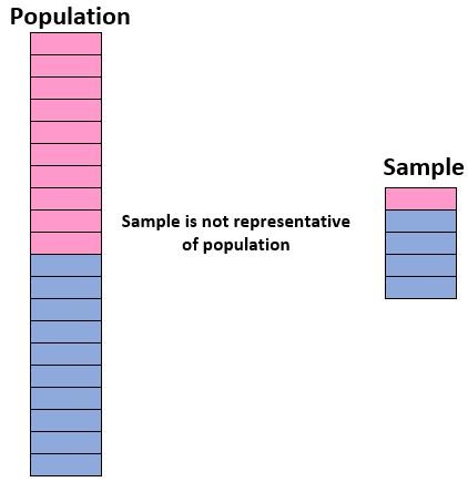
In order to be confident in our ability to use a sample to draw inferences about a population, we need to make sure that we have a representative sample – that is, a sample in which the characteristics of the individuals in the sample closely match the characteristics of the overall population.
Ideally, we want our sample to be like a “mini version” of our population. So, if we want to draw inferences on a population of students composed of 50% girls and 50% boys, our sample would not be representative if it included 90% boys and only 10% girls.

If our sample is not similar to the overall population, then we cannot generalize the findings from the sample to the overall population with any confidence.
How to Obtain a Representative Sample
To maximize the chances that you obtain a representative sample, you need to focus on two things:
1. Make sure you use a random sampling method.
There are several different random sampling methods that you can use that are likely to produce a representative sample, including:
- A simple random sample
- A systematic random sample
- A cluster random sample
- A stratified random sample
Random sampling methods tend to produce representative samples because every member of the population has an equal chance of being included in the sample.
2. Make sure your sample size is large enough.
Along with using an appropriate sampling method, it’s important to ensure that the sample is large enough so that you have enough data to generalize to the larger population.
To determine how large your sample should be, you have to consider the population size you’re studying, the confidence level you’d like to use, and the margin of error you consider to be acceptable.
Fortunately, you can use online calculators to plug in these values and see how large your sample needs to be.
Common Forms of Inferential Statistics
There are three common forms of inferential statistics:
1. Hypothesis Tests.
Often we’re interested in answering questions about a population such as:
- Is the percentage of people in Ohio in support of candidate A higher than 50%?
- Is the mean height of a certain plant equal to 14 inches?
- Is there a difference between the mean height of students at School A compared to School B?
To answer these questions we can perform a hypothesis test, which allows us to use data from a sample to draw conclusions about populations.
2. Confidence Intervals.
Sometimes we’re interested in estimating some value for a population. For example, we might be interested in the mean height of a certain plant species in Australia.
Instead of going around and measuring every single plant in the country, we might collect a small sample of plants and measure each one. Then, we can use the mean height of the plants in the sample to estimate the mean height for the population.
However, our sample is unlikely to provide a perfect estimate for the population. Fortunately, we can account for this uncertainty by creating a confidence interval, which provides a range of values that we’re confident the true population parameter falls in.
For example, we might produce a 95% confidence interval of [13.2, 14.8], which says we’re 95% confident that the true mean height of this plant species is between 13.2 inches and 14.8 inches.
3. Regression.
Sometimes we’re interested in understanding the relationship between two variables in a population.
For example, suppose we want to know if hours spent studying per week is related to test scores. To answer this question, we could perform a technique known as regression analysis.
So, we may observe the number of hours studied along with the test scores for 100 students and perform a regression analysis to see if there is a significant relationship between the two variables.
If the p-value of the regression turns out to be significant, then we can conclude that there is a significant relationship between these two variables in the overall population of students.
The Difference Between Descriptive and Inferential Statistics
In summary, the difference between descriptive and inferential statistics can be described as follows:
Descriptive statistics use summary statistics, graphs, and tables to describe a data set.
This is useful for helping us gain a quick and easy understanding of a data set without pouring over all of the individual data values.
Inferential statistics use samples to draw inferences about larger populations.
Depending on the question you want to answer about a population, you may decide to use one or more of the following methods: hypothesis tests, confidence intervals, and regression analysis.
If you do choose to use one of these methods, keep in mind that your sample needs to be representative of your population, or the conclusions you draw will be unreliable.