In statistics, deciles are numbers that split a dataset into ten groups of equal frequency.
The first decile is the point where 10% of all data values lie below it. The second decile is the point where 20% of all data values lie below it, and so forth.
We can use the following function to calculate the deciles for a dataset in Excel:
=PERCENTILE(CELL RANGE, PERCENTILE)
The following example shows how to use this function in practice.
Example: Calculate Deciles in Excel
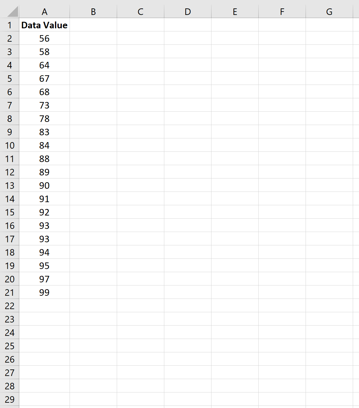
Suppose we have the following dataset with 20 values:

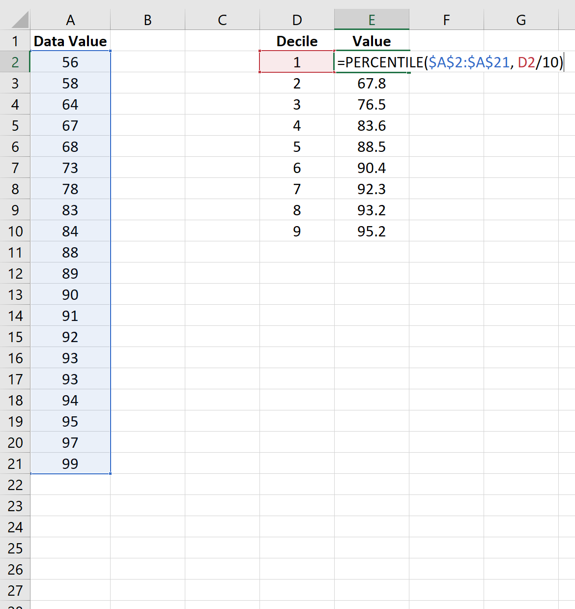
The following image shows how to calculate the deciles for the dataset:

The way to interpret the deciles is as follows:
- 20% of all data values lie below 67.8.
- 30% of all data values lie below 76.5.
- 40% of all data values lie below 83.6.
And so on.
To place each data value into a decile, we can use the PERCENTRANK.EXC() function, which uses the following syntax:
=PERCENTRANK.EXC(CELL RANGE, DATA VALUE, SIGNIFICANCE)
The following image shows how to use this function for our dataset:

Note that this function finds the relative rank of a value in a dataset as a percentage and rounds to one digit, which is equivalent to finding the decile that the value falls in.
The way to interpret the output is as follows:
- The data value 58 falls between the percentile 0 and 0.1, thus it falls in the first decile.
- The data value 64 falls between the percentile 0.1 and 0.2, thus it falls in the second decile.
- The data value 67 falls between the percentile 0.1 and 0.2, thus it falls in the second decile.
- The data value 68 falls between the percentile 0.2 and 0.3, thus it falls in the third decile.
And so on.
Additional Resources
How to Calculate a Five Number Summary in Excel
How to Normalize Data in Excel
How to Easily Find Outliers in Excel