The binomial distribution is one of the most popular distributions in statistics. To understand the binomial distribution, it helps to first understand binomial experiments.
Binomial Experiments
A binomial experiment is an experiment that has the following properties:
- The experiment consists of n repeated trials.
- Each trial has only two possible outcomes.
- The probability of success, denoted p, is the same for each trial.
- Each trial is independent.
The most obvious example of a binomial experiment is a coin flip. For example, suppose we flip a coin 10 times. This is a binomial experiment because it has the following four properties:
- The experiment consists of n repeated trials – There are 10 trials.
- Each trial has only two possible outcomes – heads or tails.
- The probability of success, denoted p, is the same for each trial – If we define “success” as landing on heads, then the probability of success is exactly 0.5 for each trial.
- Each trial is independent – The outcome of one coin flip does not affect the outcome of any other coin flip.
The Binomial Distribution
The binomial distribution describes the probability of obtaining k successes in n binomial experiments.
If a random variable X follows a binomial distribution, then the probability that X = k successes can be found by the following formula:
P(X=k) = nCk * pk * (1-p)n-k
where:
- n: number of trials
- k: number of successes
- p: probability of success on a given trial
- nCk: the number of ways to obtain k successes in n trials
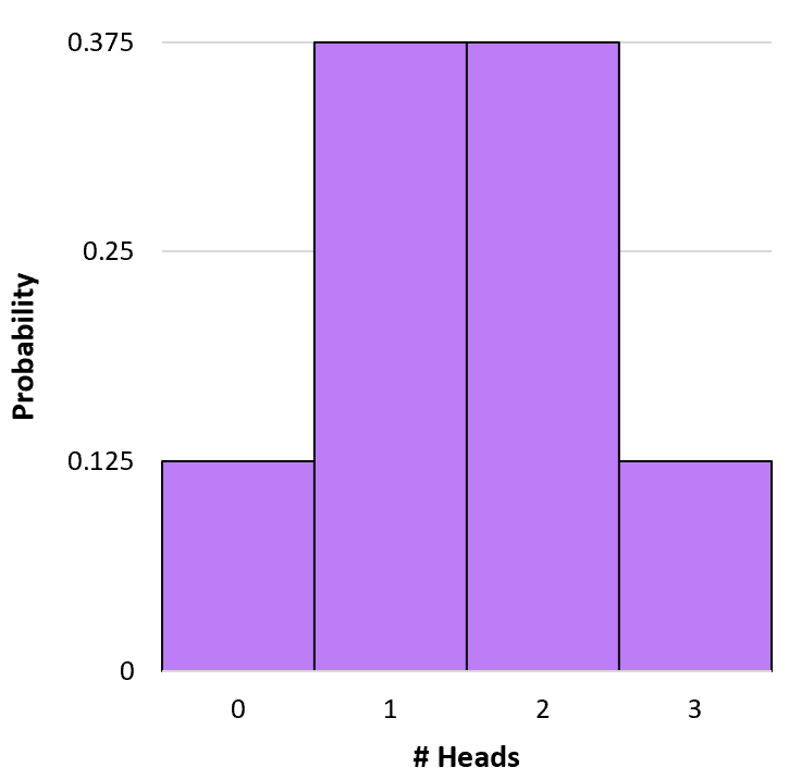
For example, suppose we flip a coin 3 times. We can use the formula above to determine the probability of obtaining 0, 1, 2, and 3 heads during these 3 flips:
P(X=0) = 3C0 * .50 * (1-.5)3-0 = 1 * 1 * (.5)3 = 0.125
P(X=1) = 3C1 * .51 * (1-.5)3-1 = 3 * .5 * (.5)2 = 0.375
P(X=2) = 3C2 * .52 * (1-.5)3-2 = 3 * .25 * (.5)1 = 0.375
P(X=3) = 3C3 * .53 * (1-.5)3-3 = 1 * .125 * (.5)0 = 0.125
Note: We used this Combination Calculator to calculate nCk for each example.
We can create a simple histogram to visualize this probability distribution:
Calculating Cumulative Binomial Probabilities
It’s straightforward to calculate a single binomial probability (e.g. the probability of a coin landing on heads 1 time out of 3 flips) using the formula above, but to calculate cumulative binomial probabilities we need to add individual probabilities.
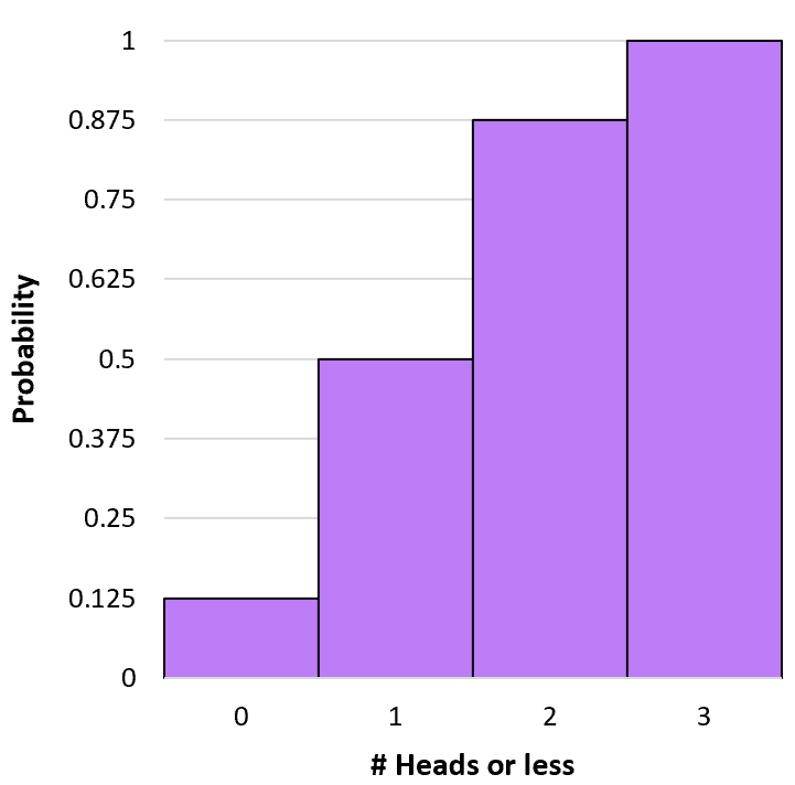
For example, suppose we want to know the probability that a coin lands on heads 1 time or less out of 3 flips. We would use the following formula to calculate this probability:
P(X≤1) = P(X=0) + P(X=1) = 0.125 + 0.375 = 0.5.
This is known as a cumulative probability because it involves adding more than one probability. We can calculate the cumulative probability of obtaining k or less heads for each outcome using a similar formula:
P(X≤0) = P(X=0) = 0.125.
P(X≤1) = P(X=0) + P(X=1) = 0.125 + 0.375 = 0.5.
P(X≤2) = P(X=0) + P(X=1) + P(X=2) = 0.125 + 0.375 + 0.375 = 0.875.
P(X≤3) = P(X=0) + P(X=1) + P(X=2) + P(X=3) = 0.125 + 0.375 + 0.375 + 0.125 = 1.
We can create a histogram to visualize this cumulative probability distribution:
Binomial Probability Calculator
When we’re working with small numbers (e.g. 3 coin flips), it’s reasonable to calculate binomial probabilities by hand. However, when we’re working with larger numbers (e.g. 100 coin flips), it can be cumbersome to calculate probabilities by hand. In these cases, it can be helpful to use a binomial probability calculator like the one below.
For example, suppose we flip a coin n = 100 times, the probability that it lands on heads in a given trial is p = 0.5, and we want to know the probability that it will land on heads k = 43 times or less:
P(X=43) = 0.03007
P(X43) = 0.06661
P(X≤43) = 0.09667
P(X>43) = 0.90333
P(X≥43) = 0.93339
Here is how to interpret the output:
- The probability that the coin lands on heads exactly 43 times is 0.03007.
- The probability that the coin lands on heads less than 43 times is 0.06661.
- The probability that the coin lands on heads 43 times or less is 0.09667.
- The probability that the coin lands on heads more than 43 times is 0.90333.
- The probability that the coin lands on heads 43 times or more is 0.93339.
Properties of the Binomial Distribution
The binomial distribution has the following properties:
The mean of the distribution is μ = np
The variance of the distribution is σ2 = np(1-p)
The standard deviation of the distribution is σ = √np(1-p)
For example, suppose we toss a coin 3 times. Let p = the probability the coin lands on heads.
The mean number of heads we would expect is μ = np = 3*.5 = 1.5.
The variance in the number of heads we would expect is σ2 = np(1-p) = 3*.5*(1-.5) = 0.75.
Binomial Distribution Practice Problems
Use the following practice problems to test your knowledge of the binomial distribution.
Problem 1
Question: Bob makes 60% of his free-throw attempts. If he shoots 12 free throws, what is the probability that he makes exactly 10?
Answer: Using the Binomial Distribution Calculator above with p = 0.6, n = 12, and k = 10, we find that P(X=10) = 0.06385.
Problem 2
Question: Jessica flips a coin 5 times. What is the probability that the coin lands on heads 2 times or fewer?
Answer: Using the Binomial Distribution Calculator above with p = 0.5, n = 5, and k = 2, we find that P(X≤2) = 0.5.
Problem 3
Question: The probability that a given student gets accepted to a certain college is 0.2. If 10 students apply, what is the probability that more than 4 get accepted?
Answer: Using the Binomial Distribution Calculator above with p = 0.2, n = 10, and k = 4, we find that P(X>4) = 0.03279.
Problem 4
Question: You flip a coin 12 times. What is the mean expected number of heads that will show up?
Answer: Recall that the mean of a binomial distribution is calculated as μ = np. Thus, μ = 12*0.5 = 6 heads.
Problem 5
Question: Mark hits a home run during 10% of his attempts. If he has 5 attempts in a given game, what is the variance of the number of home runs he’ll hit?
Answer: Recall that the variance of a binomial distribution is calculated as σ2 = np(1-p). Thus, σ2 = 6*.1*(1-.1) = 0.54.
Additional Resources
The following articles can help you learn how to work with the binomial distribution in different statistical softwares: