To apply conditional formatting to cells that are greater than or equal to some value in Excel, you can use the New Rule option under the Conditional Formatting dropdown menu within the Home tab.

The following example shows how to use this option in practice.
Example: Apply Conditional Formatting if Cell is Greater Than or Equal to Value
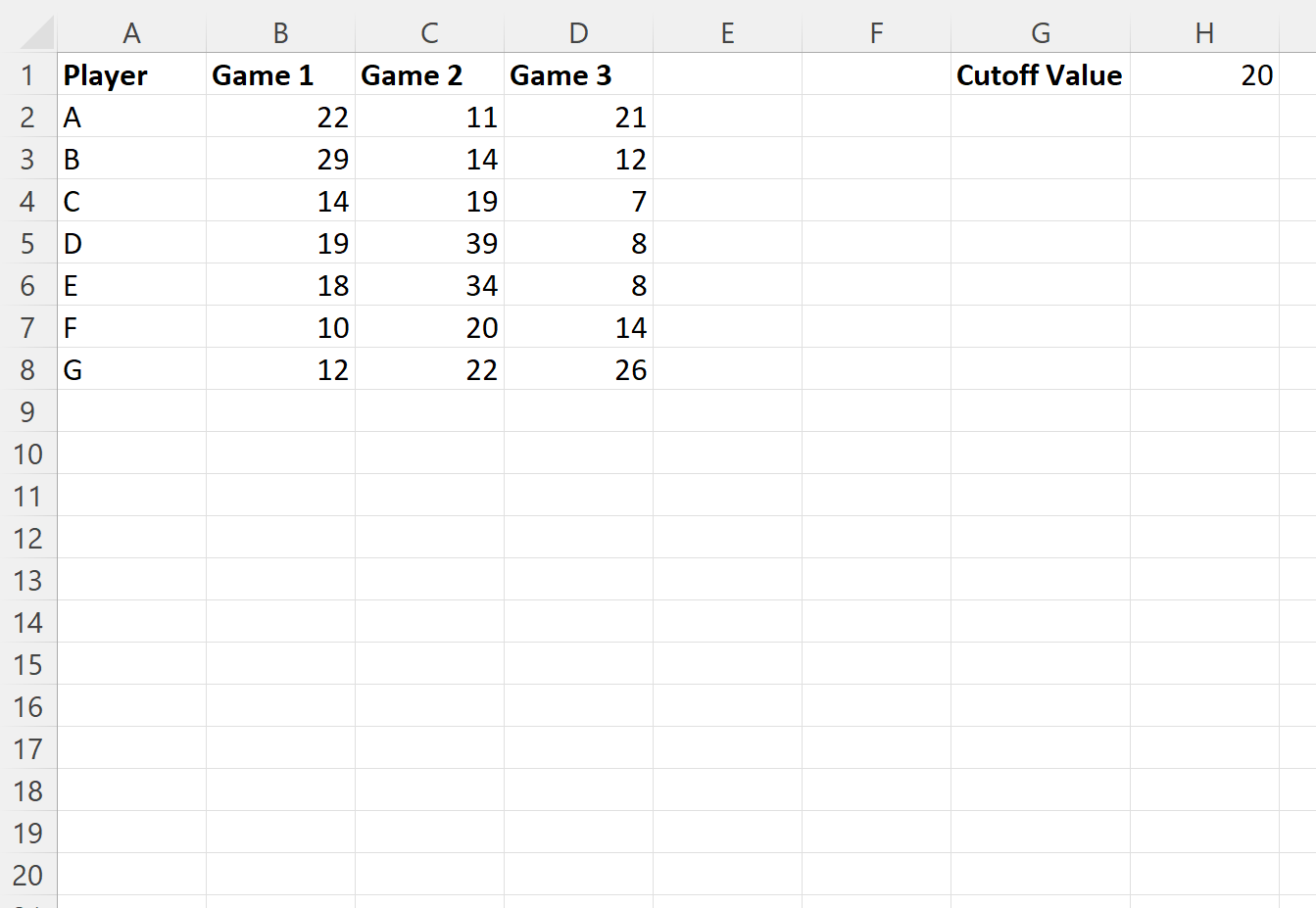
Suppose we have the following dataset in Excel that shows the number of points scored by various basketball players during three different games:

Now suppose that we would like to apply conditional formatting to each cell in the dataset that has a value greater than or equal to 20.
First, type the value 20 into cell H1:
Next, highlight the cells in the range B2:D8, then click the Conditional Formatting dropdown menu on the Home tab and then click New Rule:

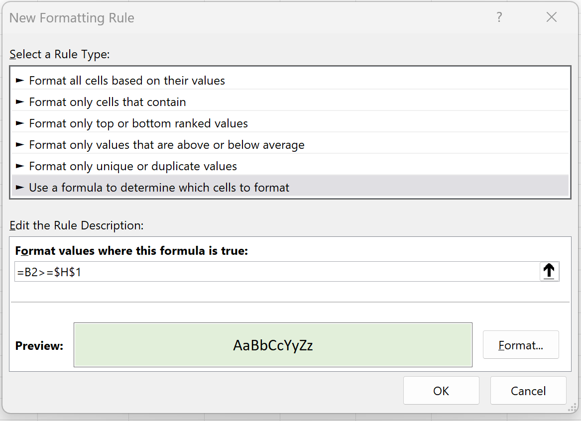
In the new window that appears, click Use a formula to determine which cells to format, then type =B2>=$H$1 in the box, then click the Format button and choose a fill color to use.
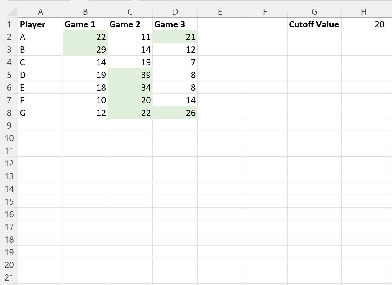
Once we press OK, all of the cells in the range B2:D8 that have a value greater than or equal to 20 will be highlighted:
If we change the cutoff value to a different number, such as 30, then the conditional formatting rule will automatically adjust to only highlight cells with a value greater than or equal to 30:
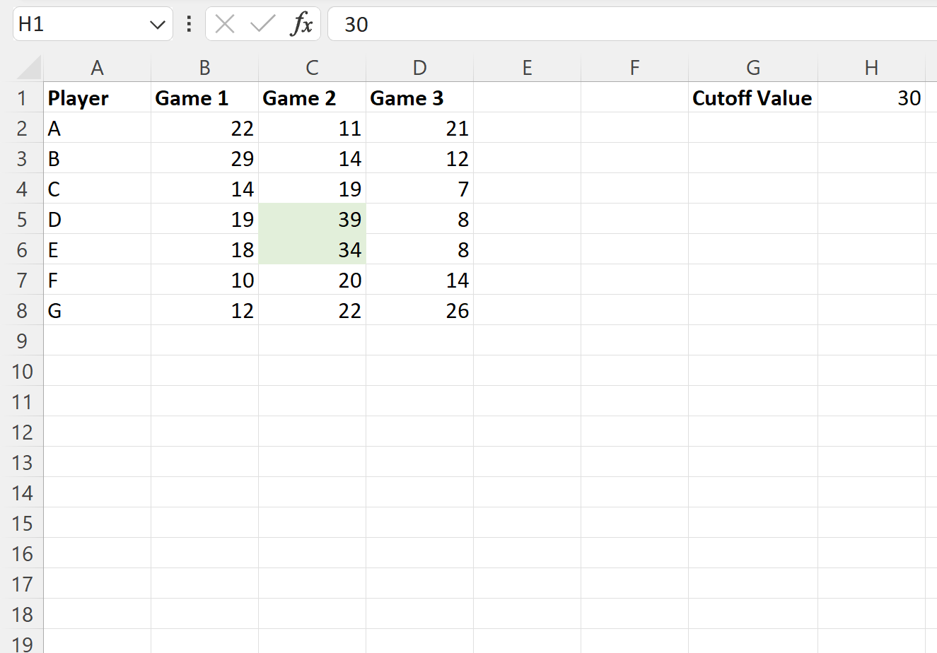
Note: We chose to use a light green fill for the conditional formatting in this example, but you can choose any color and style you’d like for the conditional formatting.
Additional Resources
The following tutorials explain how to perform other common tasks in Excel:
Excel: Apply Conditional Formatting if Cell Contains Text
Excel: Apply Conditional Formatting with Multiple Conditions
Excel: Apply Conditional Formatting if Between Two Values