Linear regression is a useful statistical method we can use to understand the relationship between two variables, x and y. However, before we conduct linear regression, we must first make sure that four assumptions are met:
1. Linear relationship: There exists a linear relationship between the independent variable, x, and the dependent variable, y.
2. Independence: The residuals are independent. In particular, there is no correlation between consecutive residuals in time series data.
3. Homoscedasticity: The residuals have constant variance at every level of x.
4. Normality: The residuals of the model are normally distributed.
If one or more of these assumptions are violated, then the results of our linear regression may be unreliable or even misleading.
In this post, we provide an explanation for each assumption, how to determine if the assumption is met, and what to do if the assumption is violated.
Assumption 1: Linear Relationship
Explanation
The first assumption of linear regression is that there is a linear relationship between the independent variable, x, and the independent variable, y.
How to determine if this assumption is met
The easiest way to detect if this assumption is met is to create a scatter plot of x vs. y. This allows you to visually see if there is a linear relationship between the two variables. If it looks like the points in the plot could fall along a straight line, then there exists some type of linear relationship between the two variables and this assumption is met.
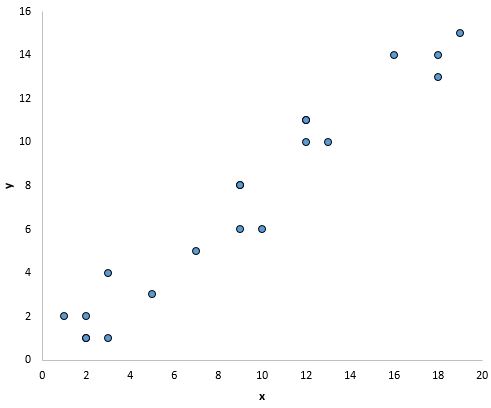
For example, the points in the plot below look like they fall on roughly a straight line, which indicates that there is a linear relationship between x and y:
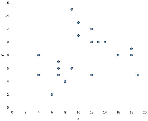
However, there doesn’t appear to be a linear relationship between x and y in the plot below:
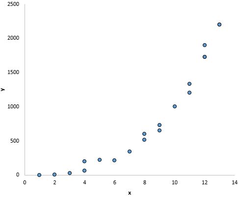
And in this plot there appears to be a clear relationship between x and y, but not a linear relationship:
What to do if this assumption is violated
If you create a scatter plot of values for x and y and see that there is not a linear relationship between the two variables, then you have a couple options:
1. Apply a nonlinear transformation to the independent and/or dependent variable. Common examples include taking the log, the square root, or the reciprocal of the independent and/or dependent variable.
2. Add another independent variable to the model. For example, if the plot of x vs. y has a parabolic shape then it might make sense to add X2 as an additional independent variable in the model.
Assumption 2: Independence
Explanation
The next assumption of linear regression is that the residuals are independent. This is mostly relevant when working with time series data. Ideally, we don’t want there to be a pattern among consecutive residuals. For example, residuals shouldn’t steadily grow larger as time goes on.
How to determine if this assumption is met
The simplest way to test if this assumption is met is to look at a residual time series plot, which is a plot of residuals vs. time. Ideally, most of the residual autocorrelations should fall within the 95% confidence bands around zero, which are located at about +/- 2-over the square root of n, where n is the sample size. You can also formally test if this assumption is met using the Durbin-Watson test.
What to do if this assumption is violated
Depending on the nature of the way this assumption is violated, you have a few options:
- For positive serial correlation, consider adding lags of the dependent and/or independent variable to the model.
- For negative serial correlation, check to make sure that none of your variables are overdifferenced.
- For seasonal correlation, consider adding seasonal dummy variables to the model.
Assumption 3: Homoscedasticity
Explanation
The next assumption of linear regression is that the residuals have constant variance at every level of x. This is known as homoscedasticity. When this is not the case, the residuals are said to suffer from heteroscedasticity.
When heteroscedasticity is present in a regression analysis, the results of the analysis become hard to trust. Specifically, heteroscedasticity increases the variance of the regression coefficient estimates, but the regression model doesn’t pick up on this. This makes it much more likely for a regression model to declare that a term in the model is statistically significant, when in fact it is not.
How to determine if this assumption is met
The simplest way to detect heteroscedasticity is by creating a fitted value vs. residual plot.
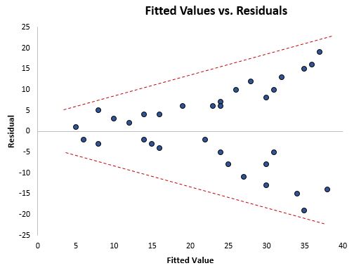
Once you fit a regression line to a set of data, you can then create a scatterplot that shows the fitted values of the model vs. the residuals of those fitted values. The scatterplot below shows a typical fitted value vs. residual plot in which heteroscedasticity is present.
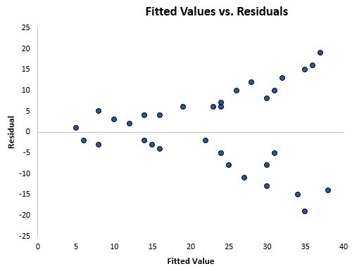
Notice how the residuals become much more spread out as the fitted values get larger. This “cone” shape is a classic sign of heteroscedasticity:
What to do if this assumption is violated
There are three common ways to fix heteroscedasticity:
1. Transform the dependent variable. One common transformation is to simply take the log of the dependent variable. For example, if we are using population size (independent variable) to predict the number of flower shops in a city (dependent variable), we may instead try to use population size to predict the log of the number of flower shops in a city. Using the log of the dependent variable, rather than the original dependent variable, often causes heteroskedasticity to go away.
2. Redefine the dependent variable. One common way to redefine the dependent variable is to use a rate, rather than the raw value. For example, instead of using the population size to predict the number of flower shops in a city, we may instead use population size to predict the number of flower shops per capita. In most cases, this reduces the variability that naturally occurs among larger populations since we’re measuring the number of flower shops per person, rather than the sheer amount of flower shops.
3. Use weighted regression. Another way to fix heteroscedasticity is to use weighted regression. This type of regression assigns a weight to each data point based on the variance of its fitted value. Essentially, this gives small weights to data points that have higher variances, which shrinks their squared residuals. When the proper weights are used, this can eliminate the problem of heteroscedasticity.
Assumption 4: Normality
Explanation
The next assumption of linear regression is that the residuals are normally distributed.
How to determine if this assumption is met
There are two common ways to check if this assumption is met:
1. Check the assumption visually using Q-Q plots.
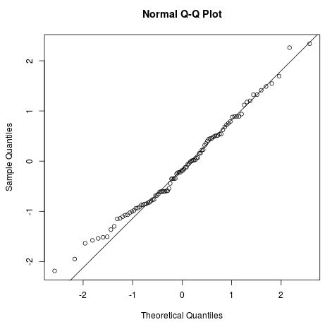
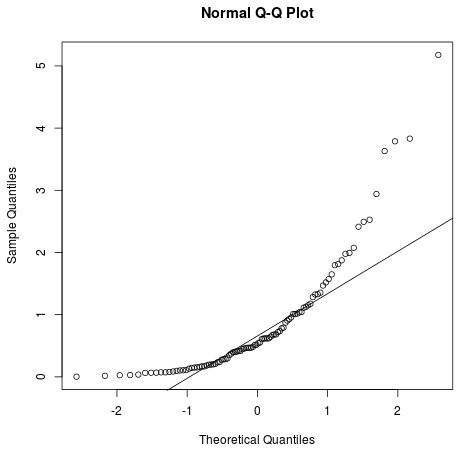
A Q-Q plot, short for quantile-quantile plot, is a type of plot that we can use to determine whether or not the residuals of a model follow a normal distribution. If the points on the plot roughly form a straight diagonal line, then the normality assumption is met.
The following Q-Q plot shows an example of residuals that roughly follow a normal distribution:
However, the Q-Q plot below shows an example of when the residuals clearly depart from a straight diagonal line, which indicates that they do not follow normal distribution:
2. You can also check the normality assumption using formal statistical tests like Shapiro-Wilk, Kolmogorov-Smironov, Jarque-Barre, or D’Agostino-Pearson. However, keep in mind that these tests are sensitive to large sample sizes – that is, they often conclude that the residuals are not normal when your sample size is large. This is why it’s often easier to just use graphical methods like a Q-Q plot to check this assumption.
What to do if this assumption is violated
If the normality assumption is violated, you have a few options:
- First, verify that any outliers aren’t having a huge impact on the distribution. If there are outliers present, make sure that they are real values and that they aren’t data entry errors.
- Next, you can apply a nonlinear transformation to the independent and/or dependent variable. Common examples include taking the log, the square root, or the reciprocal of the independent and/or dependent variable.
Further Reading:
Introduction to Simple Linear Regression
Understanding Heteroscedasticity in Regression Analysis
How to Create & Interpret a Q-Q Plot in R