Occasionally you may want to find the top 10 values in a list in Excel. Fortunately this is easy to do using the LARGE() function, which uses the following syntax:
LARGE(array, k)
where:
- array: The array of values.
- k: The kth largest value to find in the array.
This tutorial shows an example of how to use this function in practice.
Example: Find the Top 10 Values in Excel
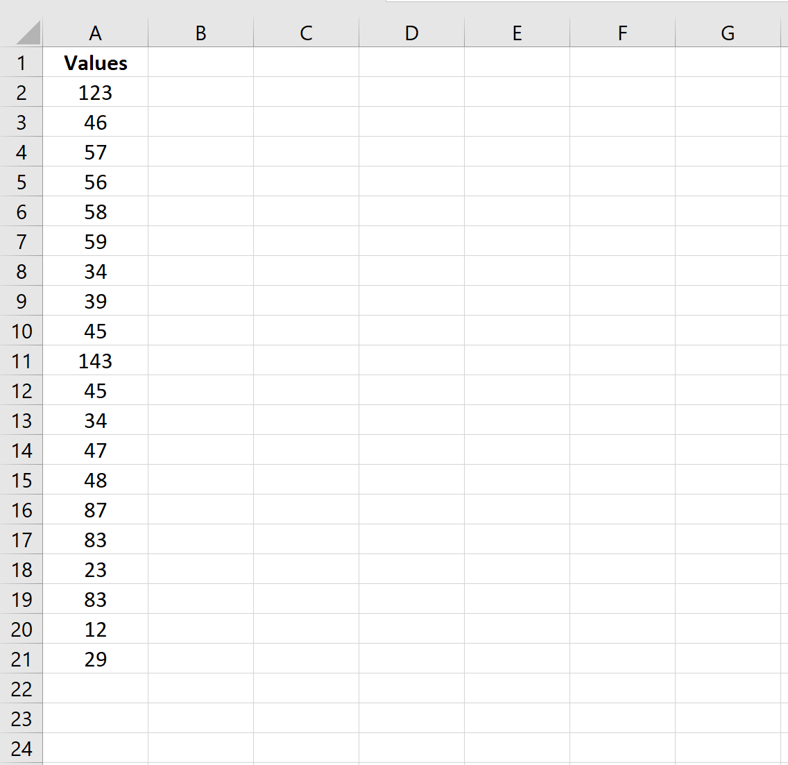
Suppose we have the following column of 20 values in Excel:

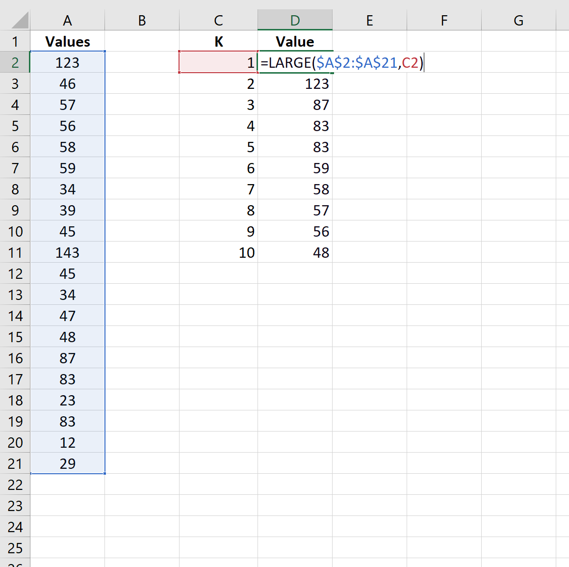
To find the 10 largest values in the list, we can create a new column titled K that lists numbers 1 through 10.
We can then create a column adjacent tot it titled Value and use the following formula to calculate the kth largest value in the dataset:
=LARGE($A$2:$A$21,C3)
We can simply copy and paste this formula down to the remaining cells in the column to find the 10 largest values in the dataset:

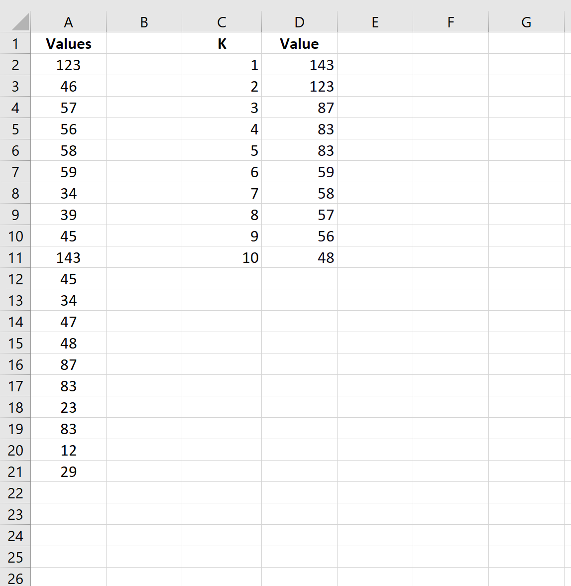
This leaves us with a list of the 10 largest values in the dataset:

We can see that the largest value is 143, the second largest is 123, the third largest is 87, and so on.
Note that we can use this method on a column of any length in Excel.
Additional Resources
How to Calculate a Five Number Summary in Excel
How to Calculate the Interquartile Range (IQR) in Excel
How to Create a Frequency Distribution in Excel