A two sample t-test is used to test whether or not the means of two populations are equal.
This tutorial explains how to conduct a two sample t-test in Stata.
Example: Two Sample t-test in Stata
Researchers want to know if a new fuel treatment leads to a change in the average mpg of a certain car. To test this, they conduct an experiment in which 12 cars receive the new fuel treatment and 12 cars do not.
Perform the following steps to conduct a two sample t-test to determine if there is a difference in average mpg between these two groups.
Step 1: Load the data.
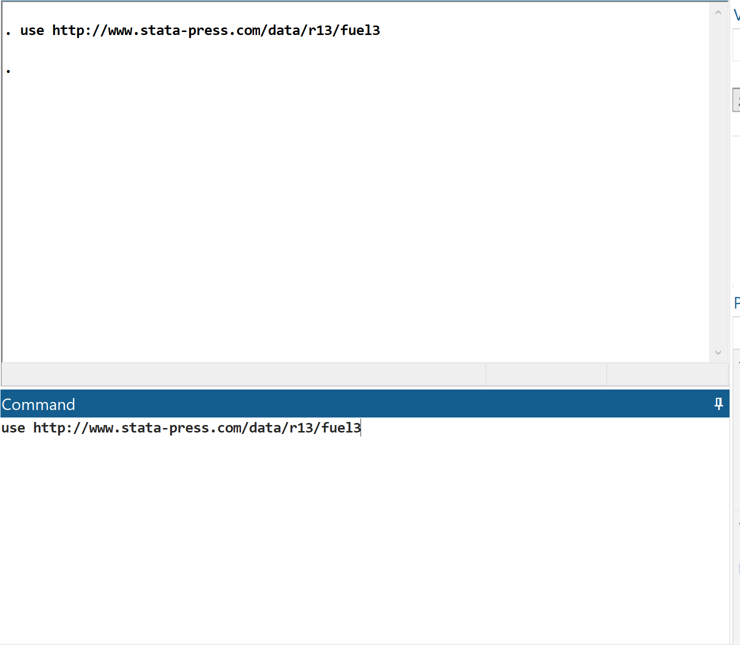
First, load the data by typing use http://www.stata-press.com/data/r13/fuel3 in the command box and clicking Enter.
Step 2: View the raw data.
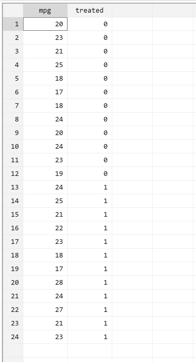
Before we perform a two sample t-test, let’s first view the raw data. Along the top menu bar, go to Data > Data Editor > Data Editor (Browse). The first column, mpg, shows the mpg for a given car. The second column, treated, indicates whether or not the car received the fuel treatment (0 = no, 1 = yes).
Step 3: Visualize the data.
Next, let’s visualize the data. We’ll create boxplots to view the distribution of mpg values for each group.
Along the top menu bar, go to Graphics > Box plot. Under variables, choose mpg:

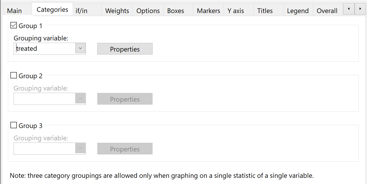
Then, in the Categories subheading under Grouping variable, choose treated:
Click OK. A chart with two boxplots will automatically be displayed:
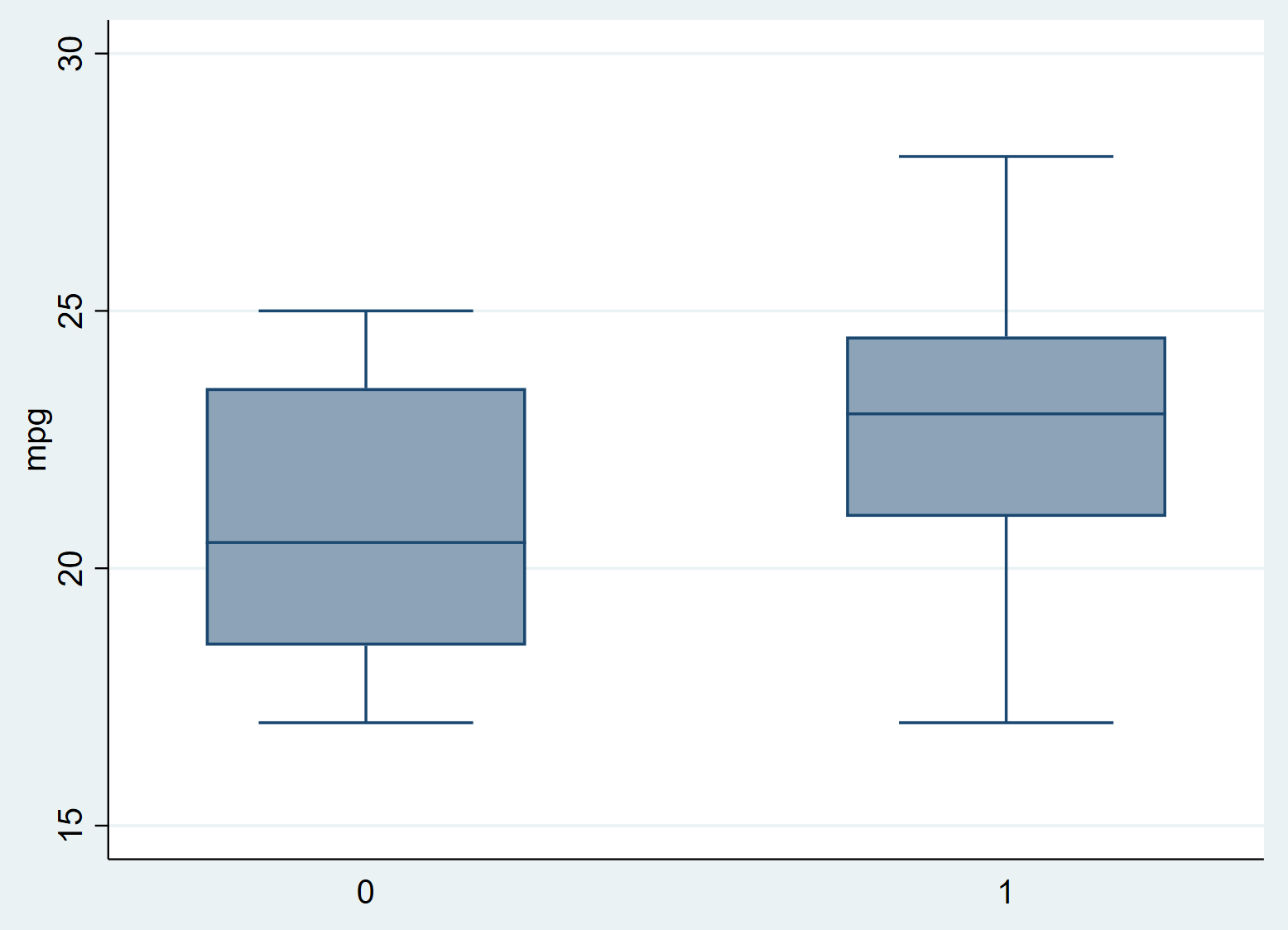
Right away we can see that the mpg appears to be higher for the treated group (1) compared to the non-treated group (0), but we need to conduct a two-sample t-test to see if these differences are statistically significant.
Step 4: Perform a two sample t-test.
Along the top menu bar, go to Statistics > Summaries, tables, and tests > Classical tests of hypotheses > t test (mean-comparison test).
Choose Two-sample using groups. For Variable name, choose mpg. For Group variable name, choose treated. For Confidence level, choose any level you’d like. A value of 95 corresponds to a significance level of 0.05. We will leave this at 95. Lastly, click OK.
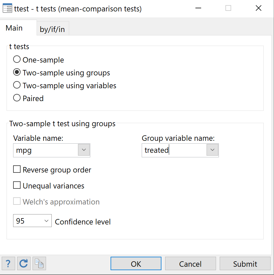
The results of the two sample t-test will be displayed:
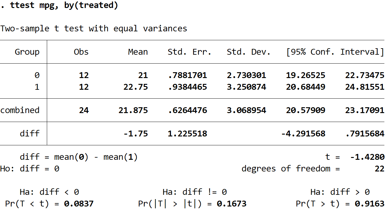
We are given the following information for each group:
Obs: The number of observations. There are 12 observations in each group.
Mean: The mean mpg. In group 0, the mean is 21. In group 1, the mean is 22.75.
Std. Err: The standard error, calculated as σ / √n
Std. Dev: The standard deviation of mpg.
95% Conf. Interval: The 95% confidence interval for the true population mean of mpg.
t: The test statistic of the two-sample t-test.
degrees of freedom: The degrees of freedom to be used for the test, calculated as n-2 = 24-2 = 22.
The p-values for three different two sample t-tests are displayed at the bottom of the results. Since we are interested in understanding if the average mpg is simply different between the two groups, we will look at the results of the middle test (in which the alternative hypothesis is Ha: diff !=0) which has a p-value of 0.1673.
Since this value is not smaller than our significance level of 0.05, we fail to reject the null hypothesis. We do not have sufficient evidence to say that the true mean mpg is different between the two groups.
Step 5: Report the results.
Lastly, we will report the results of our two sample t-test. Here is an example of how to do so:
A two sample t-test was conducted on 24 cars to determine if a new fuel treatment lead to a difference in mean miles per gallon. Each group contained 12 cars.
Results showed that the mean mpg was not different between the two groups (t = -1.428 w/ df=22, p = .1673) at a significance level of 0.05.
A 95% confidence interval for the true difference in population means resulted in the interval of (-4.29, .79).