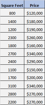
Suppose we have the following dataset that shows the square feet and price of 12 different houses:
We want to know if there is a significant relationship between square feet and price.
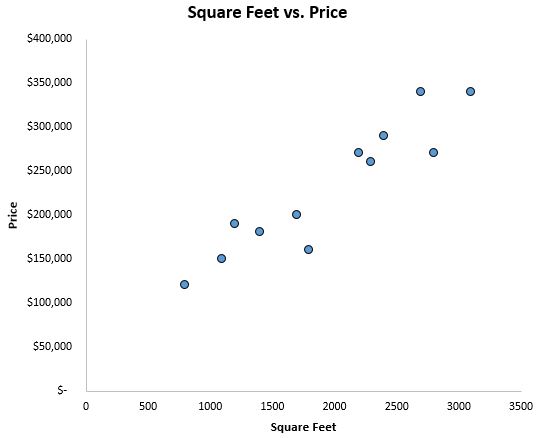
To get an idea of what the data looks like, we first create a scatterplot with square feet on the x-axis and price on the y-axis:
We can clearly see that there is a positive correlation between square feet and price. As square feet increases, the price of the house tends to increase as well.
However, to know if there is a statistically significant relationship between square feet and price, we need to run a simple linear regression.
So, we run a simple linear regression using square feet as the predictor and price as the response and get the following output:
Whether you run a simple linear regression in Excel, SPSS, R, or some other software, you will get a similar output to the one shown above.
Recall that a simple linear regression will produce the line of best fit, which is the equation for the line that best “fits” the data on our scatterplot. This line of best fit is defined as:
ŷ = b0 + b1x
where ŷ is the predicted value of the response variable, b0 is the y-intercept, b1 is the regression coefficient, and x is the value of the predictor variable.
The value for b0 is given by the coefficient for the intercept, which is 47588.70.
The value for b1 is given by the coefficient for the predictor variable Square Feet, which is 93.57.
Thus, the line of best fit in this example is ŷ = 47588.70+ 93.57x
Here is how to interpret this line of best fit:
- b0: When the value for square feet is zero, the average expected value for price is $47,588.70. (In this case, it doesn’t really make sense to interpret the intercept, since a house can never have zero square feet)
- b1: For each additional square foot, the average expected increase in price is $93.57.
So, now we know that for each additional square foot, the average expected increase in price is $93.57.
To find out if this increase is statistically significant, we need to conduct a hypothesis test for B1 or construct a confidence interval for B1.
Note: A hypothesis test and a confidence interval will always give the same results.
Constructing a Confidence Interval for a Regression Slope
To construct a confidence interval for a regression slope, we use the following formula:
Confidence Interval = b1 +/- (t1-∝/2, n-2) * (standard error of b1)
where:
- b1 is the slope coefficient given in the regression output
- (t1-∝/2, n-2) is the t critical value for confidence level 1-∝ with n-2 degrees of freedom where n is the total number of observations in our dataset
- (standard error of b1) is the standard error of b1 given in the regression output
For our example, here is how to construct a 95% confidence interval for B1:
- b1 is 93.57 from the regression output.
- Since we are using a 95% confidence interval, ∝ = .05 and n-2 = 12-2 = 10, thus t.975, 10 is 2.228 according to the t-distribution table
- (standard error of b1) is 11.45 from the regression output
Thus, our 95% confidence interval for B1 is:
93.57 +/- (2.228) * (11.45) = (68.06 , 119.08)
This means we are 95% confident that the true average increase in price for each additional square foot is between $68.06 and $119.08.
Notice that $0 is not in this interval, so the relationship between square feet and price is statistically significant at the 95% confidence level.
Conducting a Hypothesis Test for a Regression Slope
To conduct a hypothesis test for a regression slope, we follow the standard five steps for any hypothesis test:
Step 1. State the hypotheses.
The null hypothesis (H0): B1 = 0
The alternative hypothesis: (Ha): B1 ≠ 0
Step 2. Determine a significance level to use.
Since we constructed a 95% confidence interval in the previous example, we will use the equivalent approach here and choose to use a .05 level of significance.
Step 3. Find the test statistic and the corresponding p-value.
In this case, the test statistic is t = coefficient of b1 / standard error of b1 with n-2 degrees of freedom. We can find these values from the regression output:

Thus, test statistic t = 92.89 / 13.88 = 6.69.
Using the T Score to P Value Calculator with a t score of 6.69 with 10 degrees of freedom and a two-tailed test, the p-value = 0.000.
Step 4. Reject or fail to reject the null hypothesis.
Since the p-value is less than our significance level of .05, we reject the null hypothesis.
Step 5. Interpret the results.
Since we rejected the null hypothesis, we have sufficient evidence to say that the true average increase in price for each additional square foot is not zero.


