A studentized residual is simply a residual divided by its estimated standard deviation.
In practice, we typically say that any observation in a dataset that has a studentized residual greater than an absolute value of 3 is an outlier.
We can quickly obtain the studentized residuals of any regression model in R by using the studres() function from the MASS package, which uses the following syntax:
studres(model)
where model represents any linear model.
Example: Calculating Studentized Residuals in R
Suppose we build the following simple linear regression model in R, using the built-in mtcars dataset:
#build simple linear regression model
model
We can use the studres() function from the MASS package to calculate the studentized residuals for each observation in the dataset:
library(MASS)

#calculate studentized residuals
stud_resids #view first three studentized residuals
head(stud_resids, 3)

    Mazda RX4 Mazda RX4 Wag    Datsun 710
   -0.6236250    -0.6236250    -0.7405315
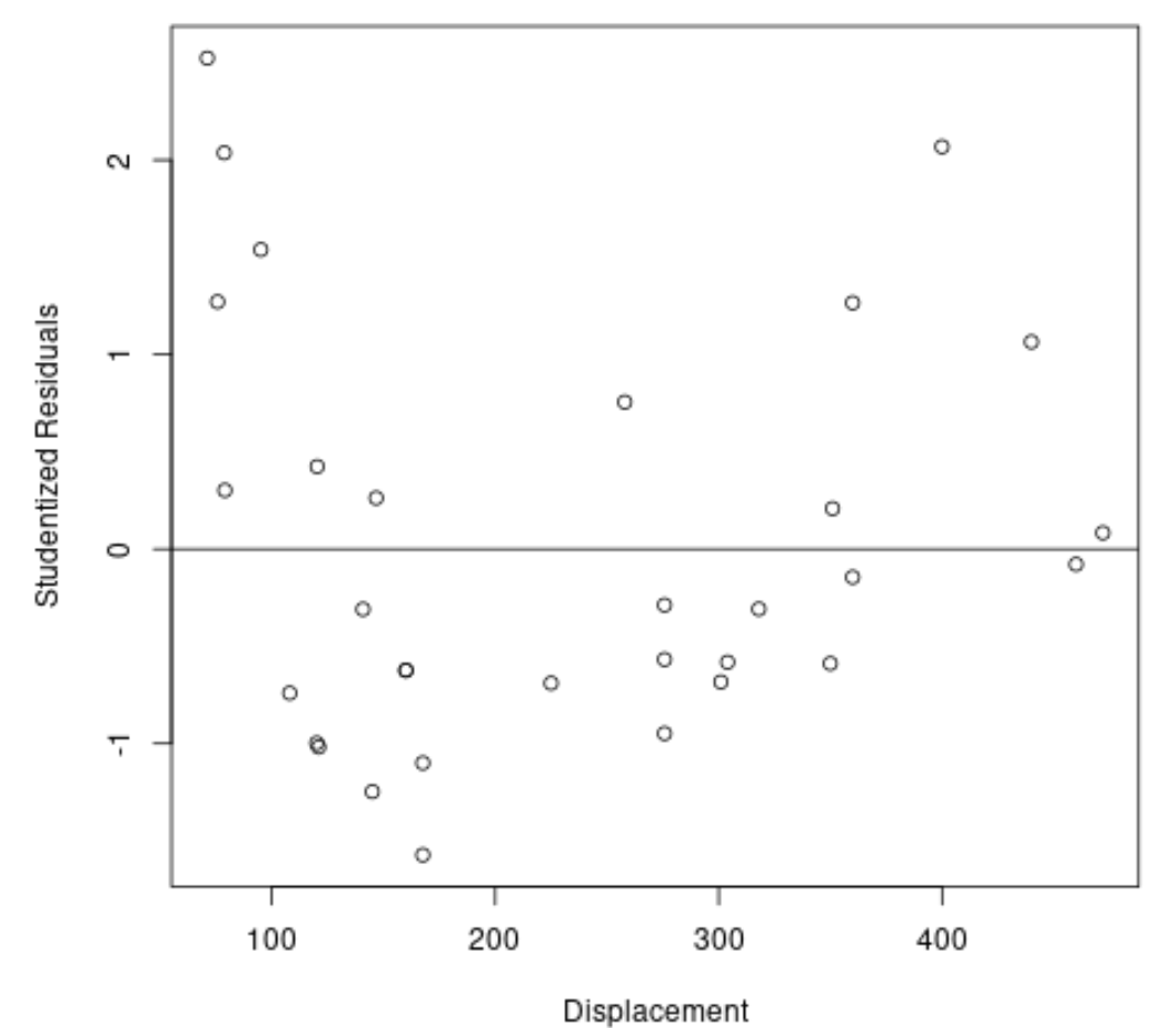
We can also create a quick plot of the predictor variable values vs. the corresponding studentized residuals:
#plot predictor variable vs. studentized residuals
plot(mtcars$disp, stud_resids,  ylab='Studentized Residuals', xlab='Displacement')

#add horizontal line at 0
abline(0, 0)

From the plot we can see that none of the observations have a studentized residual with an absolute value greater than 3, thus there are no clear outliers in the dataset.
We can also add the studentized residuals of each observation back into the original dataset if we’d like:
#add studentized residuals to orignal dataset
final_data cbind(mtcars[c('mpg', 'disp')], stud_resids)

#view final dataset
head(final_data)

                   mpg disp stud_resids
Mazda RX4         21.0  160  -0.6236250
Mazda RX4 Wag     21.0  160  -0.6236250
Datsun 710        22.8  108  -0.7405315
Hornet 4 Drive    21.4  258   0.7556078
Hornet Sportabout 18.7  360   1.2658336
Valiant           18.1  225  -0.6896297
We can then sort each observation from largest to smallest according to its studentized residual to get an idea of which observations are closest to being outliers:
#sort studentized residuals descending
final_data[order(-stud_resids),]

                     mpg  disp stud_resids
Toyota Corolla      33.9  71.1  2.52397102
Pontiac Firebird    19.2 400.0  2.06825391
Fiat 128            32.4  78.7  2.03684699
Lotus Europa        30.4  95.1  1.53905536
Honda Civic         30.4  75.7  1.27099586
Hornet Sportabout   18.7 360.0  1.26583364
Chrysler Imperial   14.7 440.0  1.06486066
Hornet 4 Drive      21.4 258.0  0.75560776
Porsche 914-2       26.0 120.3  0.42424678
Fiat X1-9           27.3  79.0  0.30183728
Merc 240D           24.4 146.7  0.26235893
Ford Pantera L      15.8 351.0  0.20825609
Cadillac Fleetwood  10.4 472.0  0.08338531
Lincoln Continental 10.4 460.0 -0.07863385
Duster 360          14.3 360.0 -0.14476167
Merc 450SL          17.3 275.8 -0.28759769
Dodge Challenger    15.5 318.0 -0.30826585
Merc 230            22.8 140.8 -0.30945955
Merc 450SE          16.4 275.8 -0.56742476
AMC Javelin         15.2 304.0 -0.58138205
Camaro Z28          13.3 350.0 -0.58848471
Mazda RX4 Wag       21.0 160.0 -0.62362497
Mazda RX4           21.0 160.0 -0.62362497
Maserati Bora       15.0 301.0 -0.68315010
Valiant             18.1 225.0 -0.68962974
Datsun 710          22.8 108.0 -0.74053152
Merc 450SLC         15.2 275.8 -0.94814699
Toyota Corona       21.5 120.1 -0.99751166
Volvo 142E          21.4 121.0 -1.01790487
Merc 280            19.2 167.6 -1.09979261
Ferrari Dino        19.7 145.0 -1.24732999
Merc 280C           17.8 167.6 -1.57258064
Additional Resources
How to Perform Simple Linear Regression in R
How to Perform Multiple Linear Regression in R
How to Create a Residual Plot in R