How to Calculate Standardized Residuals in R

A residual is the difference between an observed value and a predicted value in a regression model.

It is calculated as:

Residual = Observed value – Predicted value

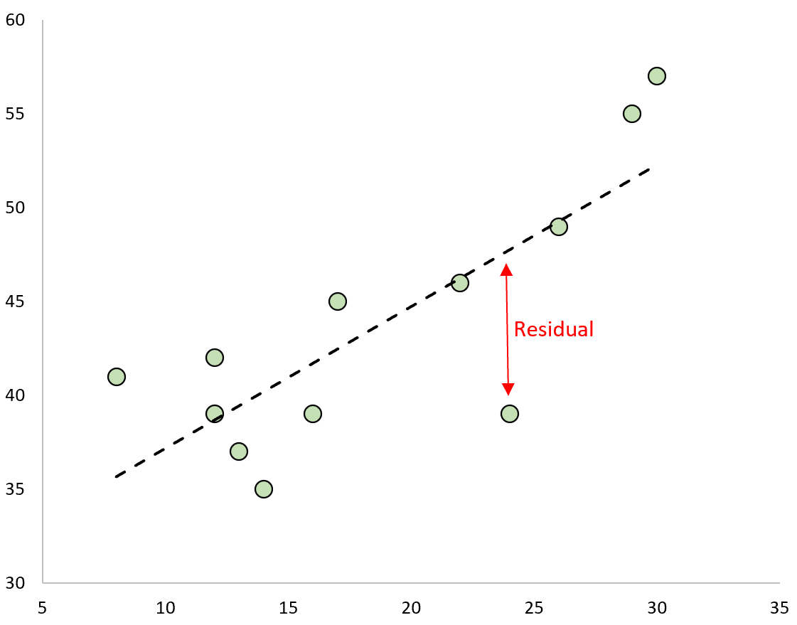
If we plot the observed values and overlay the fitted regression line, the residuals for each observation would be the vertical distance between the observation and the regression line:

One type of residual we often use to identify outliers in a regression model is known as a standardized residual.

It is calculated as:

r_i  =  e_i / s(e_i)  =  e_i / RSE√1-h_ii

where:

• e_i: The i^th residual
• RSE: The residual standard error of the model
• h_ii: The leverage of the i^th observation

In practice, we often consider any standardized residual with an absolute value greater than 3 to be an outlier.

This tutorial provides a step-by-step example of how to calculate standardized residuals in R.

Step 1: Enter the Data

First, we’ll create a small dataset to work with in R:

#create data
data #view data
data

    x  y
1   8 41
2  12 42
3  12 39
4  13 37
5  14 35
6  16 39
7  17 45
8  22 46
9  24 39
10 26 49
11 29 55
12 30 57

Step 2: Fit the Regression Model

Next, we’ll use the lm() function to fit a simple linear regression model:

#fit model
model #view model summary
summary(model) 

Call:
lm(formula = y ~ x, data = data)

Residuals:
    Min      1Q  Median      3Q     Max 
-8.7578 -2.5161  0.0292  3.3457  5.3268 

Coefficients:
            Estimate Std. Error t value Pr(>|t|)    
(Intercept)  29.6309     3.6189   8.188  9.6e-06 ***
x             0.7553     0.1821   4.148  0.00199 ** 
---
Signif. codes:  0 ‘***’ 0.001 ‘**’ 0.01 ‘*’ 0.05 ‘.’ 0.1 ‘ ’ 1

Residual standard error: 4.442 on 10 degrees of freedom
Multiple R-squared:  0.6324,	Adjusted R-squared:  0.5956 
F-statistic:  17.2 on 1 and 10 DF,  p-value: 0.001988

Step 3: Calculate the Standardized Residuals

Next, we’ll use the built-in rstandard() function to calculate the standardized residuals of the model:

#calculate the standardized residuals
standard_res #view the standardized residuals
standard_res

          1           2           3           4           5           6 
 1.40517322  0.81017562  0.07491009 -0.59323342 -1.24820530 -0.64248883 
          7           8           9          10          11          12 
 0.59610905 -0.05876884 -2.11711982 -0.06655600  0.91057211  1.26973888

We can add the standardized residuals back to the original data frame if we’d like:

#column bind standardized residuals back to original data frame
final_data #view data frame
    x  y standard_res
1   8 41   1.40517322
2  12 42   0.81017562
3  12 39   0.07491009
4  13 37  -0.59323342
5  14 35  -1.24820530
6  16 39  -0.64248883
7  17 45   0.59610905
8  22 46  -0.05876884
9  24 39  -2.11711982
10 26 49  -0.06655600
11 29 55   0.91057211
12 30 57   1.26973888

We can then sort each observation from largest to smallest according to its standardized residual to get an idea of which observations are closest to being outliers:

#sort standardized residuals descending
final_data[order(-standard_res),]

    x  y standard_res
1   8 41   1.40517322
12 30 57   1.26973888
11 29 55   0.91057211
2  12 42   0.81017562
7  17 45   0.59610905
3  12 39   0.07491009
8  22 46  -0.05876884
10 26 49  -0.06655600
4  13 37  -0.59323342
6  16 39  -0.64248883
5  14 35  -1.24820530
9  24 39  -2.11711982

From the results we can see that none of the standardized residuals exceed an absolute value of 3. Thus, none of the observations appear to be outliers.

Step 4: Visualize the Standardized Residuals

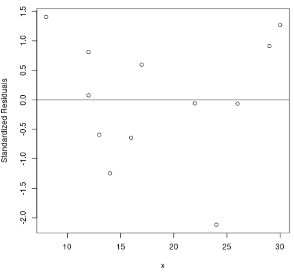
Lastly, we can create a scatterplot to visualize the values for the predictor variable vs. the standardized residuals:

#plot predictor variable vs. standardized residuals
plot(final_data$x, standard_res, ylab='Standardized Residuals', xlab='x') 

#add horizontal line at 0
abline(0, 0)

Additional Resources

What Are Residuals?
What Are Standardized Residuals?
Introduction to Multiple Linear Regression