Simple linear regression is a method we can use to understand the relationship between a predictor variable and a response variable.
This tutorial explains how to perform simple linear regression in SPSS.
Example: Simple Linear Regression in SPSS
Suppose we have the following dataset that shows the number of hours studied and the exam score received by 20 students:

Use the following steps to perform simple linear regression on this dataset to quantify the relationship between hours studied and exam score:
Step 1: Visualize the data.
First, we’ll create a scatterplot to visualize the relationship between hours and score to make sure that the relationship between the two variables appears to be linear. Otherwise, simple linear regression won’t be an appropriate technique to use.
Click the Graphs tab, then click Chart Builder:

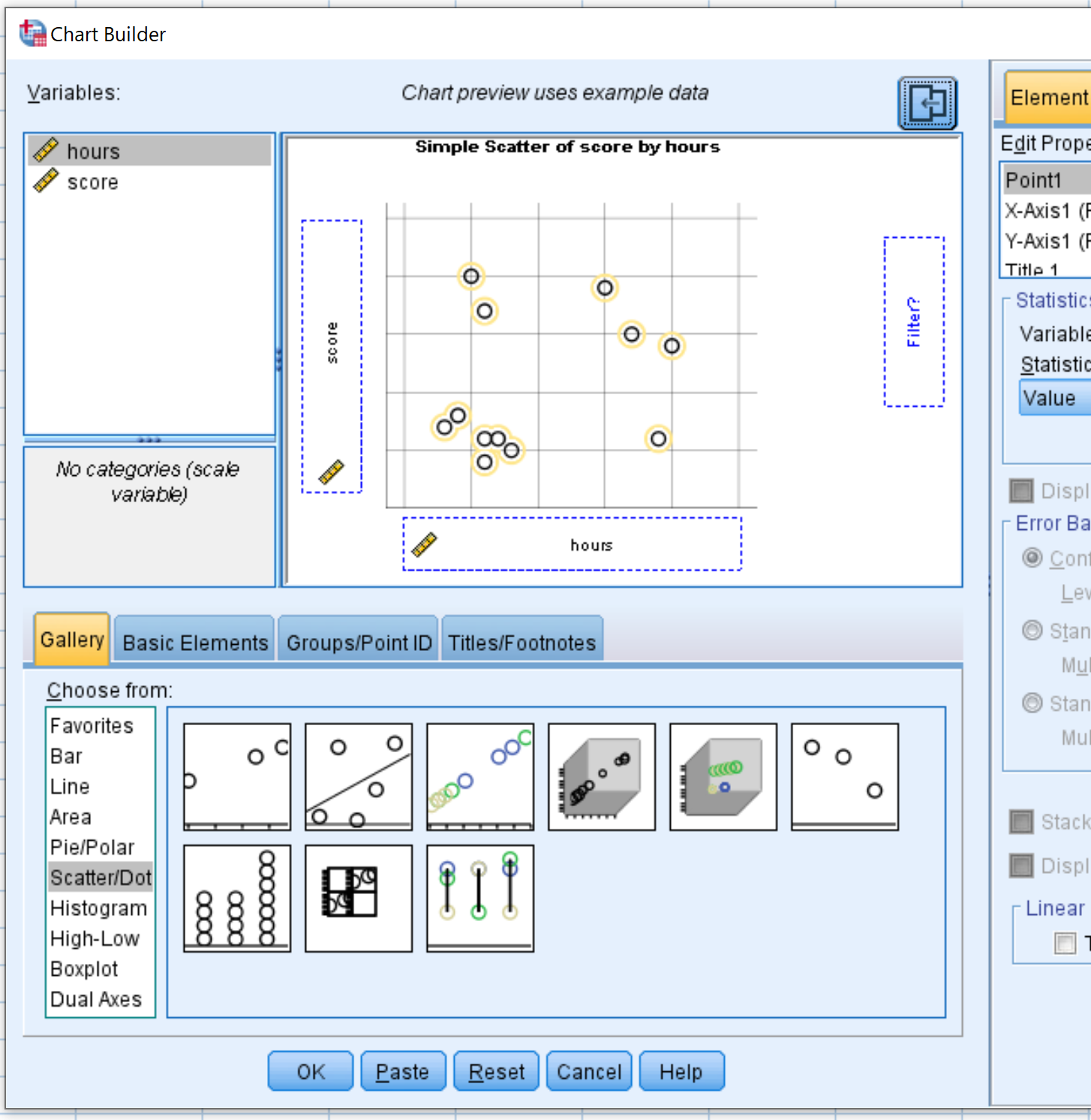
In the Choose from menu, click and drag Scatter/Dot into the main editing window. Then drag the variable hours onto the x-axis and score onto the y-axis.

Once you click OK, the following scatterplot will appear:

From the plot we can see that there is a positive linear relationship between hours and score. In general, students who study for more hours tend to get higher scores.
Since there’s a clear linear relationship between the two variables, we’ll proceed to fit a simple linear regression model to the dataset.
Step 2: Fit a simple linear regression model.
Click the Analyze tab, then Regression, then Linear:

In the new window that pops up, drag the variable score into the box labelled Dependent and drag hours into the box labelled Independent. Then click OK.

Step 3: Interpret the results.
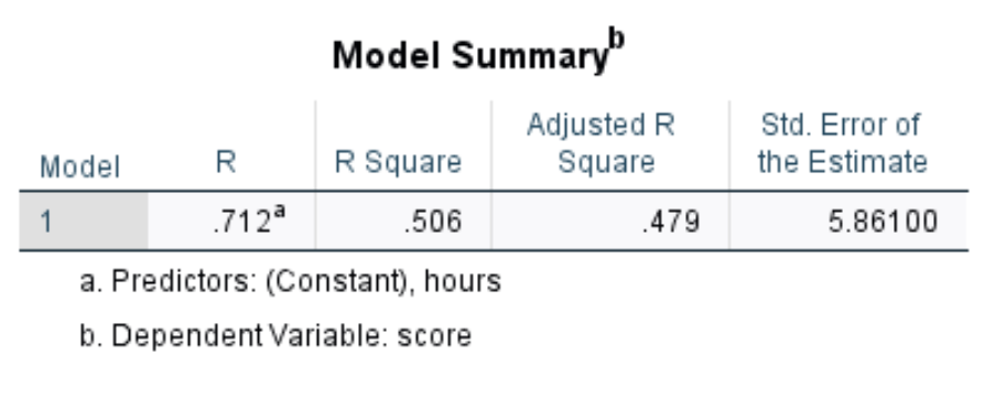
Once you click OK, the results of the simple linear regression will appear. The first table we’re interested in is the one titled Model Summary:

Here is how to interpret the most relevant numbers in this table:
- R Square: This is the proportion of the variance in the response variable that can be explained by the explanatory variable. In this example, 50.6% of the variation in exam scores can be explained by hours studied.
- Std. Error of the Estimate: The standard error is the average distance that the observed values fall from the regression line. In this example, the observed values fall an average of 5.861 units from the regression line.
The next table we’re interested in is titled Coefficients:

Here is how to interpret the most relevant numbers in this table:
- Unstandardized B (Constant): This tells us the average value of the response variable when the predictor variable is zero. In this example, the average exam score is 73.662 when hours studied is equal to zero.
- Unstandardized B (hours): This tells us the average change in the response variable associated with a one unit increase in the predictor variable. In this example, each additional hour studied is associated with an increase of 3.342 in exam score, on average.
- Sig (hours): This is the p-value associated with the test statistic for hours. In this case, since this value is less than 0.05, we can conclude that the predictor variable hours is statistically significant.
Lastly, we can form a regression equation using the values for constant and hours. In this case, the equation would be:
Estimated exam score = 73.662 + 3.342*(hours)
We can use this equation to find the estimated exam score for a student, based on the number of hours they studied. For example, a student that studies for 3 hours is expected to receive an exam score of 83.688:
Estimated exam score = 73.662 + 3.342*(3) = 83.688
Step 4: Report the results.
Lastly, we want to summarize the results of our simple linear regression. Here’s an example of how to do so:
A simple linear regression was performed to quantify the relationship between hours studied and exam score received. A sample of 20 students was used in the analysis.
Results showed that there was a statistically significant relationship between hours studied and exam score (t = 4.297, p
The regression equation was found to be:
Estimated exam score = 73.662 + 3.342*(hours)
Each additional hour studied is associated with an increase of 3.342 in exam score, on average.