A repeated measures ANOVA is used to determine whether or not there is a statistically significant difference between the means of three or more groups in which the same subjects show up in each group.
This tutorial explains how to conduct a one-way repeated measures ANOVA in SPSS.
Example: Repeated Measures ANOVA in SPSS
Researchers want to know if four different drugs lead to different reaction times. To test this, they measure the reaction time of five patients on the four different drugs. Since each patient is measured on each of the four drugs, we will use a repeated measures ANOVA to determine if the mean reaction time differs between drugs.
Perform the following steps to conduct the repeated measures ANOVA in SPSS.
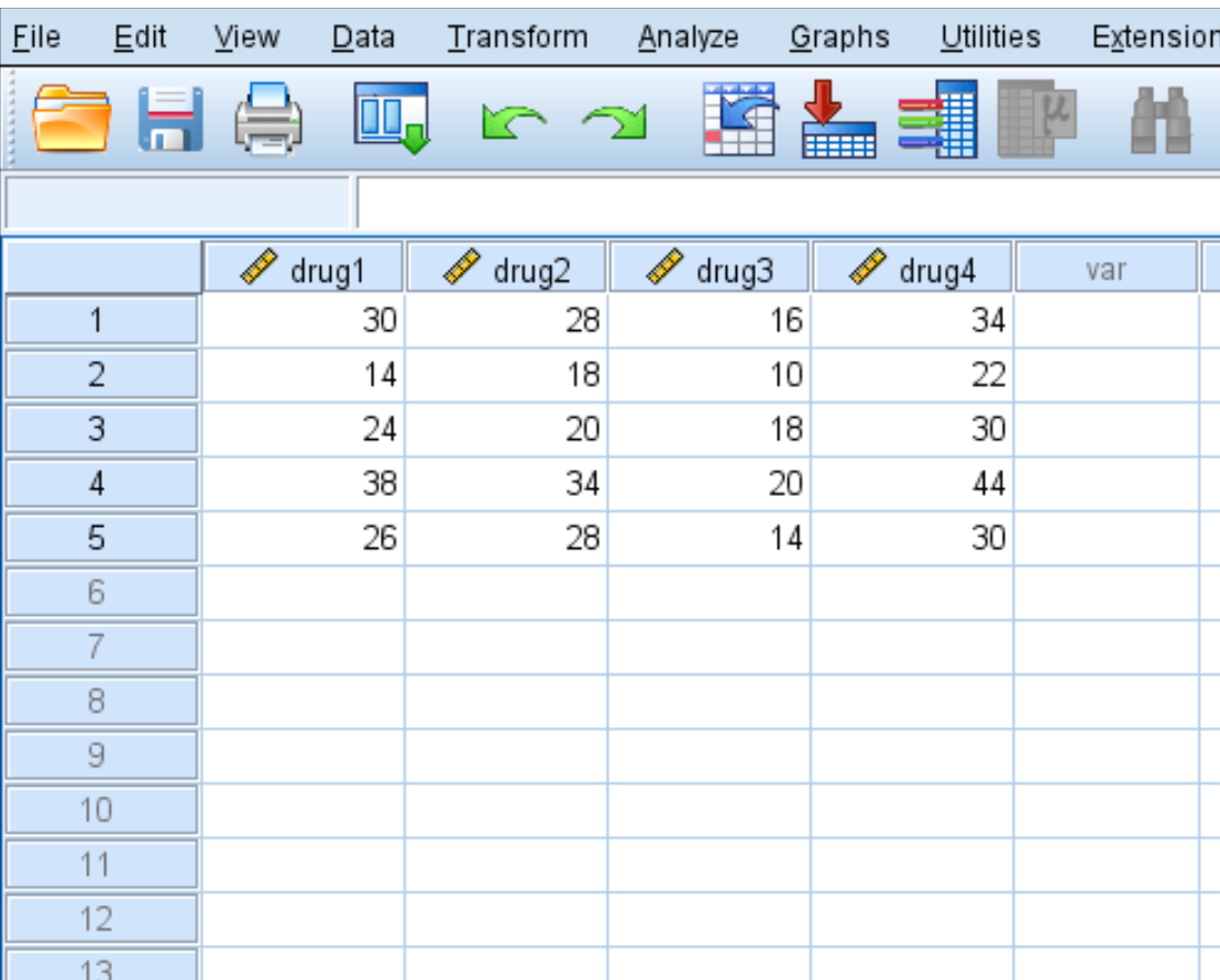
Step 1: Enter the data.
Enter the following data, which shows the response time (in seconds) of five patients on the four drugs:
Step 2: Perform a repeated measures ANOVA.
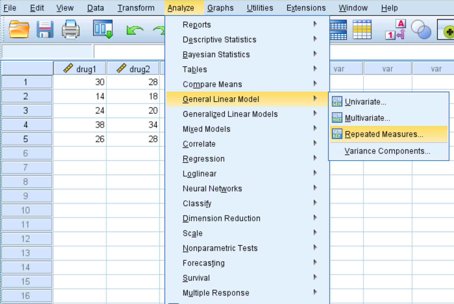
Click the Analyze tab, then General Linear Model, then Repeated Measures:
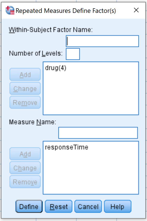
In the new window that pops up, type in the drug for the Within-Subject Factor Name. Type in 4 for the Number of Levels (since each subject in the study tested 4 different drugs), then click Add. Type in responseTime for the Measure Name, then click Add. Lastly, click Define.
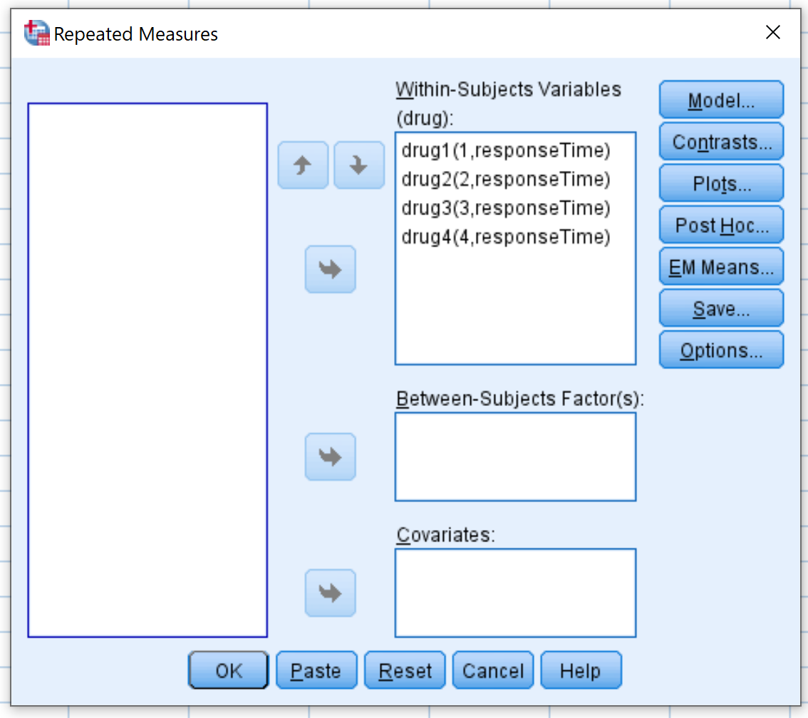
In the new window that pops up, drag each of the four drug variables into the box labelled Within-Subjects Variables:
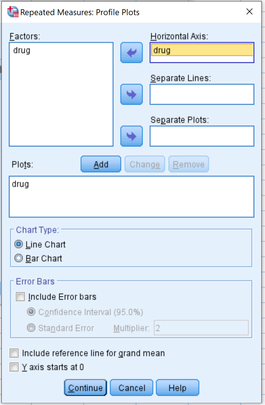
Next, click Plots. Drag the variable drug into the box labelled Horizontal Axis. Then click Add. Then click Continue.
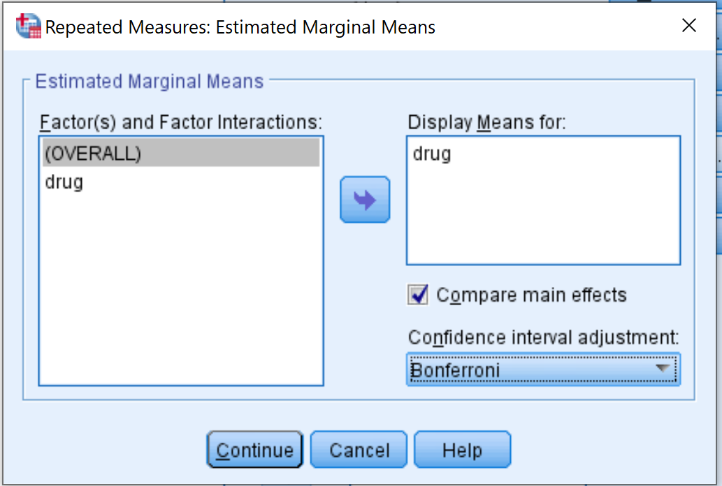
Next, click EM Means. Drag the variable drug into the box labelled Display Means for. Then check the box next to Compare main effects and select Bonferroni from the dropdown menu. Then click Continue.
Lastly, click OK.
Step 2: Interpret the results.
Once you click OK, the results of the repeated measures ANOVA will appear. Here is how to interpret the output:
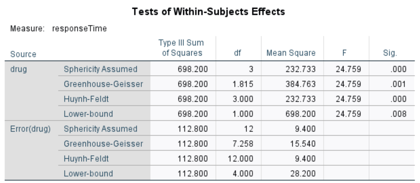
Tests of Within-Subjects Effects
This table displays the overall F-statistic and the corresponding p-value of the repeated measures ANOVA. Typically we use the values in the row titled Greenhouse-Geisser.
According to this row, the F-statistic is 24.759 and the corresponding p-value is .001. Since this p-value is less than .05, we can reject the null hypothesis and conclude that there is a statistically significant difference in mean response times between the four drugs.
Pairwise Comparisons
Since we rejected the null hypothesis, it means that at least two of the group means are different. To determine which group means are different, we can use this table that displays the pairwise comparisons between each drug.
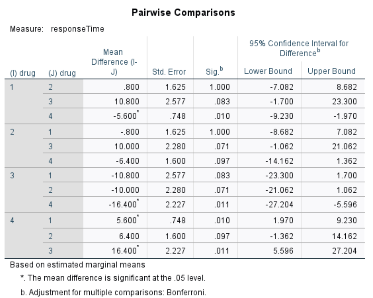
From the table we can see the p-values for the following comparisons:
- drug 1 vs. drug 2 | p-value = 1.000
- drug 1 vs. drug 3 | p-value = .083
- drug 1 vs. drug 4 | p-value = .010
- drug 2 vs. drug 3 | p-value = .071
- drug 2 vs. drug 4 | p-value = .097
- drug 3 vs. drug 4 | p-value = .011
The only p-values below .05 are for drug 1 vs. drug 4 and drug 3 vs. drug 4. All of the other comparisons have p-values greater than .05.
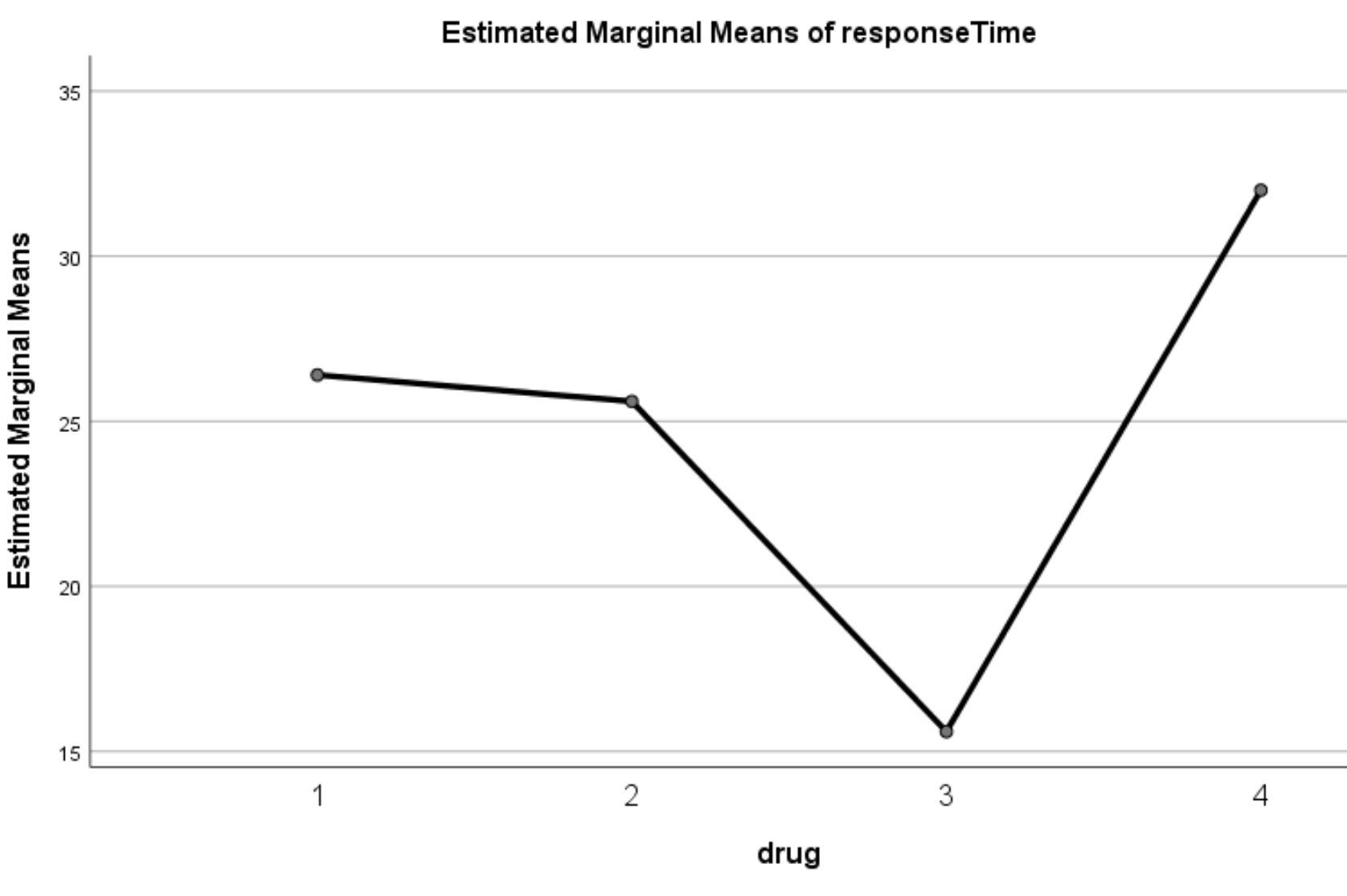
Plot of Estimated Marginal Means
This plot displays the estimated mean response times for each drug. From the plot we can clearly see that response times varied noticeably between the four different drugs:
Step 3: Report the results.
Lastly, we can report the results of the repeated measures ANOVA. Here is an example of how to do so:
A one-way repeated measures ANOVA was performed to determine if the mean reaction time in patients differed between four different drugs.
A one-way repeated measures ANOVA revealed that the type of drug used lead to statistically significant differences in response time (F = 24.75887, p = 0.001).
Bonferroni’s test for multiple comparisons found that there was a statistically significant difference in response times between patients on drug 1 vs. drug 4 along with drug 3 vs. drug 4.