You can use the following formula to perform a Percentile IF function in Excel:
=PERCENTILE(IF(GROUP_RANGE=GROUP, VALUES_RANGE), k)
This formula finds the kth percentile of all values that belong to a certain group.
When you type this formula into a cell in Google Sheets, you need to press Ctrl + Shift + Enter since this is an array formula.
The following example shows how to use this function in practice.
Example: Percentile IF Function in Google Sheets
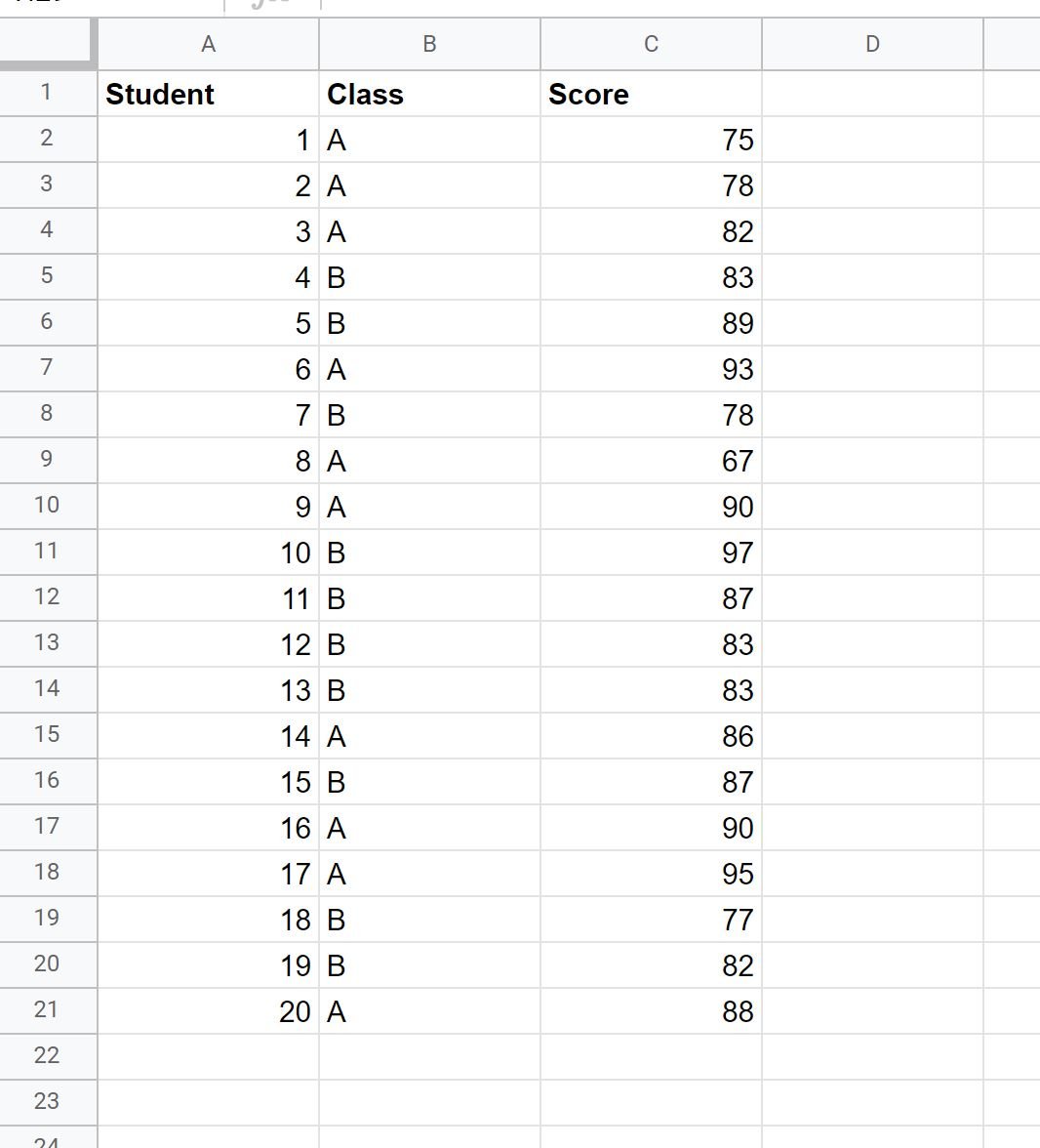
Suppose we have the following dataset that shows the exam score received by 20 students who belong to either class A or class B:
Now suppose we’d like to find the 90th percentile of the exam scores only among students who were in class A.
To do so, we can type the following formula into cell F2:
=PERCENTILE(IF(B2:B21=E2, C2:C21), 0.9)
Once we press Ctrl + Shift + Enter, the 90th percentile of exam scores among students in class A will be shown:
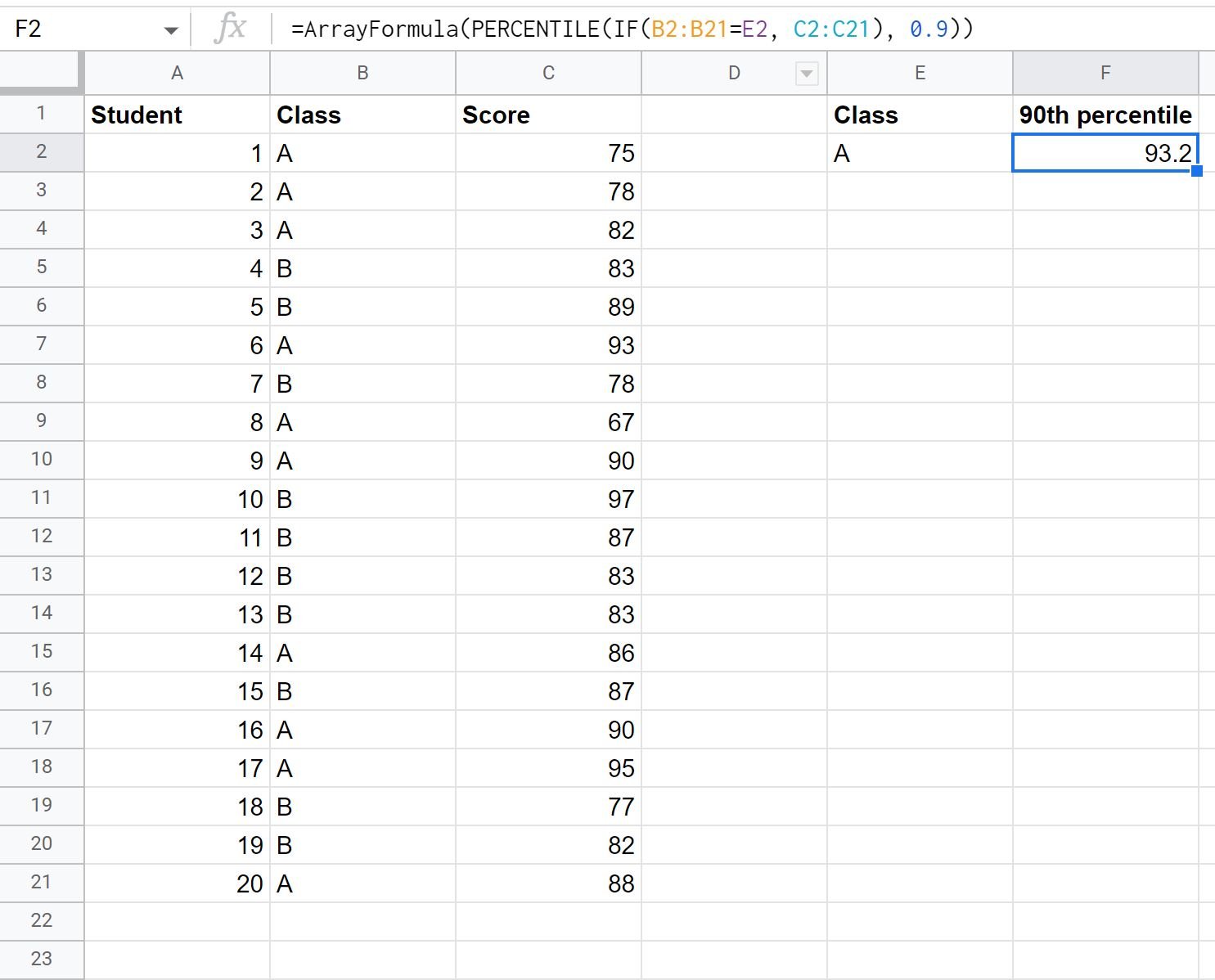
From the output we can see the value at the 90th percentile of exam scores in class A was 93.2.
To calculate the 90th percentile of exam scores for class B, we can simply change the value in cell E2.
The formula will automatically calculated the 90th percentile of exam scores among students in class B:
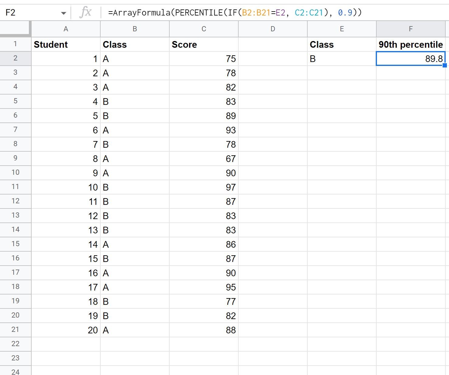
We can see that the value at the 90th percentile of exam scores in class B was 89.8.
Note that in these examples we chose to calculate the 90th percentile, but you can calculate any percentile you’d like.
For example, to calculate the 75th percentile of exam scores for each class you can replace 0.9 with 0.75 in the formula.
Additional Resources
The following tutorials explain how to perform other common tasks in Google Sheets:
How to Calculate a Five Number Summary in Google Sheets
How to Calculate Mean and Standard Deviation in Google Sheets
How to Calculate Deciles in Google Sheets