Ordinary least squares (OLS) regression is a method that allows us to find a line that best describes the relationship between one or more predictor variables and a response variable.
This method allows us to find the following equation:
ŷ = b0 + b1x
where:
- ŷ: The estimated response value
- b0: The intercept of the regression line
- b1: The slope of the regression line
This equation can help us understand the relationship between the predictor and response variable, and it can be used to predict the value of a response variable given the value of the predictor variable.
The following step-by-step example shows how to perform OLS regression in Python.
Step 1: Create the Data
For this example, we’ll create a dataset that contains the following two variables for 15 students:
- Total hours studied
- Exam score
We’ll perform OLS regression, using hours as the predictor variable and exam score as the response variable.
The following code shows how to create this fake dataset in pandas:
import pandas as pd

#create DataFrame
df = pd.DataFrame({'hours': [1, 2, 4, 5, 5, 6, 6, 7, 8, 10, 11, 11, 12, 12, 14],
                   'score': [64, 66, 76, 73, 74, 81, 83, 82, 80, 88, 84, 82, 91, 93, 89]})

#view DataFrame
print(df)

    hours  score
0       1     64
1       2     66
2       4     76
3       5     73
4       5     74
5       6     81
6       6     83
7       7     82
8       8     80
9      10     88
10     11     84
11     11     82
12     12     91
13     12     93
14     14     89
Step 2: Perform OLS Regression
Next, we can use functions from the statsmodels module to perform OLS regression, using hours as the predictor variable and score as the response variable:
import statsmodels.api as sm

#define predictor and response variables
y = df['score']
x = df['hours']

#add constant to predictor variables
x = sm.add_constant(x)

#fit linear regression model
model = sm.OLS(y, x).fit()

#view model summary
print(model.summary())

                            OLS Regression Results
==============================================================================
Dep. Variable:                  score   R-squared:                       0.831
Model:                            OLS   Adj. R-squared:                  0.818
Method:                 Least Squares   F-statistic:                     63.91
Date:                Fri, 26 Aug 2022   Prob (F-statistic):           2.25e-06
Time:                        10:42:24   Log-Likelihood:                -39.594
No. Observations:                  15   AIC:                             83.19
Df Residuals:                      13   BIC:                             84.60
Df Model:                           1
Covariance Type:            nonrobust
==============================================================================
                 coef    std err          t      P>|t|      [0.025      0.975]
------------------------------------------------------------------------------
const         65.3340      2.106     31.023      0.000      60.784      69.884
hours          1.9824      0.248      7.995      0.000       1.447       2.518
==============================================================================
Omnibus:                        4.351   Durbin-Watson:                   1.677
Prob(Omnibus):                  0.114   Jarque-Bera (JB):                1.329
Skew:                           0.092   Prob(JB):                        0.515
Kurtosis:                       1.554   Cond. No.                         19.2
==============================================================================
From the coef column we can see the regression coefficients and can write the following fitted regression equation is:
Score = 65.334 + 1.9824*(hours)
This means that each additional hour studied is associated with an average increase in exam score of 1.9824 points.
The intercept value of 65.334 tells us the average expected exam score for a student who studies zero hours.
We can also use this equation to find the expected exam score based on the number of hours that a student studies.
For example, a student who studies for 10 hours is expected to receive an exam score of 85.158:
Score = 65.334 + 1.9824*(10) = 85.158
Here is how to interpret the rest of the model summary:
- P(>|t|): This is the p-value associated with the model coefficients. Since the p-value for hours (0.000) is less than .05, we can say that there is a statistically significant association between hours and score.
- R-squared: This tells us the percentage of the variation in the exam scores can be explained by the number of hours studied. In this case, 83.1% of the variation in scores can be explained hours studied.
- F-statistic & p-value: The F-statistic (63.91) and the corresponding p-value (2.25e-06) tell us the overall significance of the regression model, i.e. whether predictor variables in the model are useful for explaining the variation in the response variable. Since the p-value in this example is less than .05, our model is statistically significant and hours is deemed to be useful for explaining the variation in score.
Step 3: Visualize the Line of Best Fit
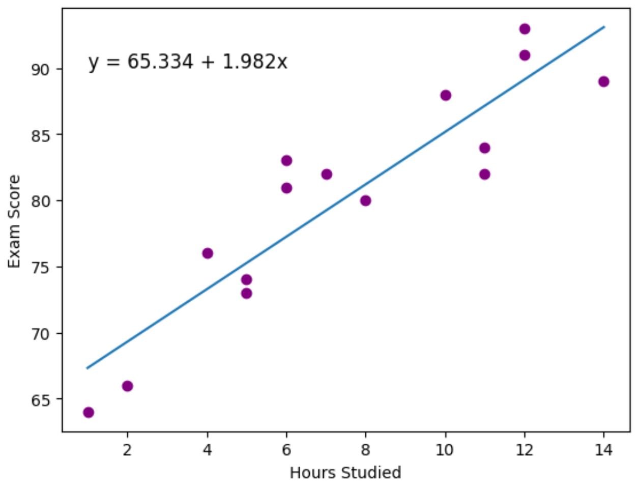
Lastly, we can use the matplotlib data visualization package to visualize the fitted regression line over the actual data points:
import matplotlib.pyplot as plt

#find line of best fit
a, b = np.polyfit(df['hours'], df['score'], 1)

#add points to plot
plt.scatter(df['hours'], df['score'], color='purple')

#add line of best fit to plot
plt.plot(df['hours'], a*df['hours']+b)

#add fitted regression equation to plot
plt.text(1, 90, 'y = ' + '{:.3f}'.format(b) + ' + {:.3f}'.format(a) + 'x', size=12)

#add axis labels
plt.xlabel('Hours Studied')
plt.ylabel('Exam Score')

The purple points represent the actual data points and the blue line represents the fitted regression line.
We also used the plt.text() function to add the fitted regression equation to the top left corner of the plot.
From looking at the plot, it looks like the fitted regression line does a pretty good job of capturing the relationship between the hours variable and the score variable.
Additional Resources
The following tutorials explain how to perform other common tasks in Python:
How to Perform Logistic Regression in Python
How to Perform Exponential Regression in Python
How to Calculate AIC of Regression Models in Python