You can use the MAXIFS function in Google Sheets to find the max value in a range, filtered by a set of criteria.
This function uses the following basic syntax:
=MAXIFS(range, criteria_range1, criteria1, [criteria_range2, criteria2, …])
The following examples show how to use this syntax in practice.
Example 1: Use MAXIFS with One Criterion
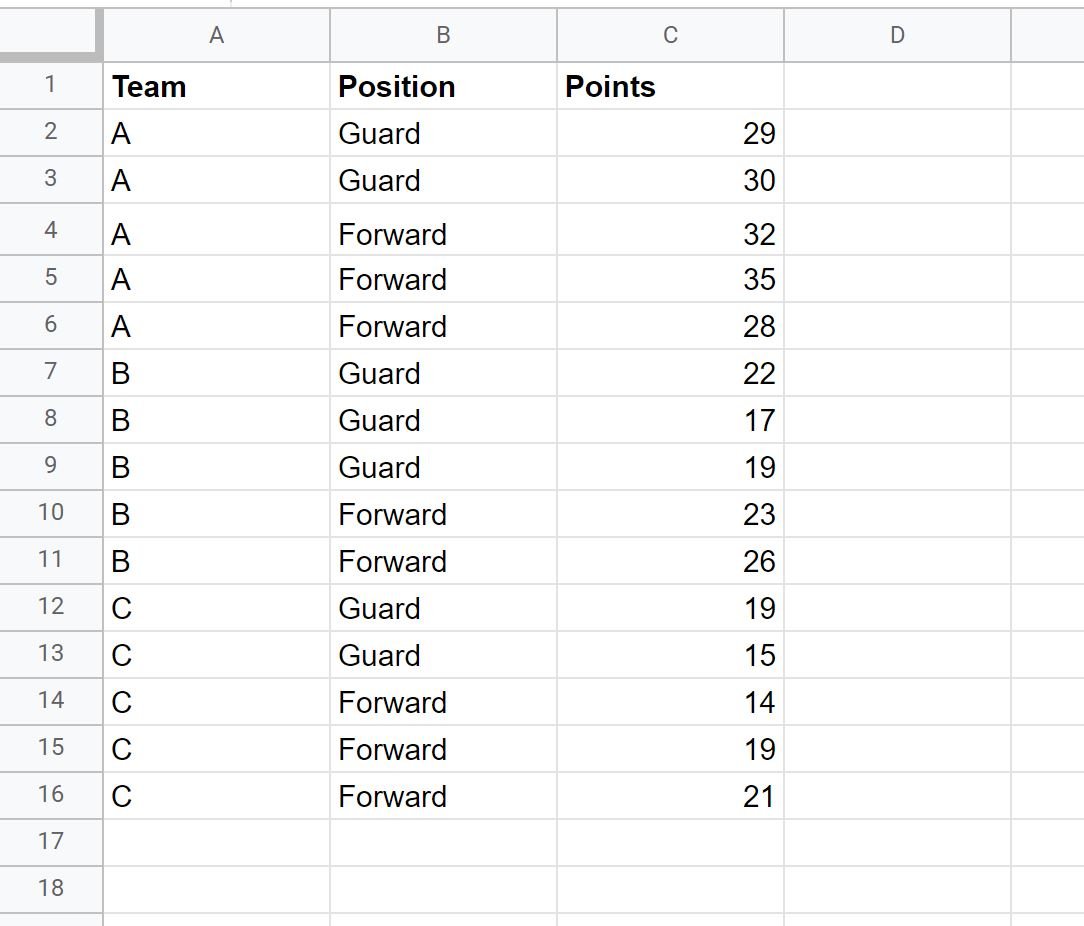
Suppose we have the following dataset that shows the points scored by 15 different basketball players:
We can use the following formula to calculate the max points scored IF the player is on team A:
=MAXIFS(C2:C16, A2:A16, "A")
The following screenshot shows how to use this formula in practice:

We can see that the max points value among players on team A is 35.
Example 2: Use MAXIFS with Multiple Criteria
Suppose we have the same dataset that shows the points scored by 15 different basketball players:
We can use the following formula to calculate the max points scored IF the player is on team A and IF the player has a Guard position:
=MAXIFS(C2:C16, A2:A16, "A", B2:B16, "Guard")
The following screenshot shows how to use this formula in practice:
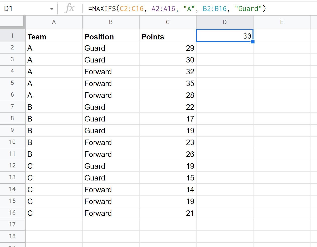
We can see that the max points value among players who are on team A and have a Guard position is 30.
Note: In these examples we used the MAXIFS() function with one criterion and two criterion, but you can use the same syntax to use as many criterion as you’d like.
Additional Resources
The following tutorials explain how to perform other common operations in Google Sheets:
How to Use COUNTIF with Multiple Ranges in Google Sheets
How to Use SUMIF with Multiple Columns in Google Sheets
How to Sum Across Multiple Sheets in Google Sheets