The lm() function in R is used to fit linear regression models.
This function uses the following basic syntax:
lm(formula, data, …)
where:
- formula: The formula for the linear model (e.g. y ~ x1 + x2)
- data: The name of the data frame that contains the data
The following example shows how to use this function in R to do the following:
- Fit a regression model
- View the summary of the regression model fit
- View the diagnostic plots for the model
- Plot the fitted regression model
- Make predictions using the regression model
Fit Regression Model
The following code shows how to use the lm() function to fit a linear regression model in R:
#define data
df = data.frame(x=c(1, 3, 3, 4, 5, 5, 6, 8, 9, 12),
                y=c(12, 14, 14, 13, 17, 19, 22, 26, 24, 22))

#fit linear regression model using 'x' as predictor and 'y' as response variable
model
View Summary of Regression Model
We can then use the summary() function to view the summary of the regression model fit:
#view summary of regression model
summary(model)

Call:
lm(formula = y ~ x, data = df)

Residuals:
    Min      1Q  Median      3Q     Max
-4.4793 -0.9772 -0.4772  1.4388  4.6328

Coefficients:
            Estimate Std. Error t value Pr(>|t|)
(Intercept)  11.1432     1.9104   5.833  0.00039 ***
x             1.2780     0.2984   4.284  0.00267 **
---
Signif. codes:  0 ‘***’ 0.001 ‘**’ 0.01 ‘*’ 0.05 ‘.’ 0.1 ‘ ’ 1

Residual standard error: 2.929 on 8 degrees of freedom
Multiple R-squared:  0.6964,	Adjusted R-squared:  0.6584
F-statistic: 18.35 on 1 and 8 DF,  p-value: 0.002675
Here’s how to interpret the most important values in the model:
- F-statistic = 18.35, corresponding p-value = .002675. Since this p-value is less than .05, the model as a whole is statistically significant.
- Multiple R-squared = .6964. This tells us that 69.64% of the variation in the response variable, y, can be explained by the predictor variable, x.
- Coefficient estimate of x: 1.2780. This tells us that each additional one unit increase in x is associated with an average increase of 1.2780 in y.
We can then use the coefficient estimates from the output to write the estimated regression equation:
y = 11.1432 + 1.2780*(x)
Bonus: You can find a complete guide to interpreting every value in the regression output in R here.
View Diagnostic Plots of Model
We can then use the plot() function to plot the diagnostic plots for the regression model:
#create diagnostic plots
plot(model)
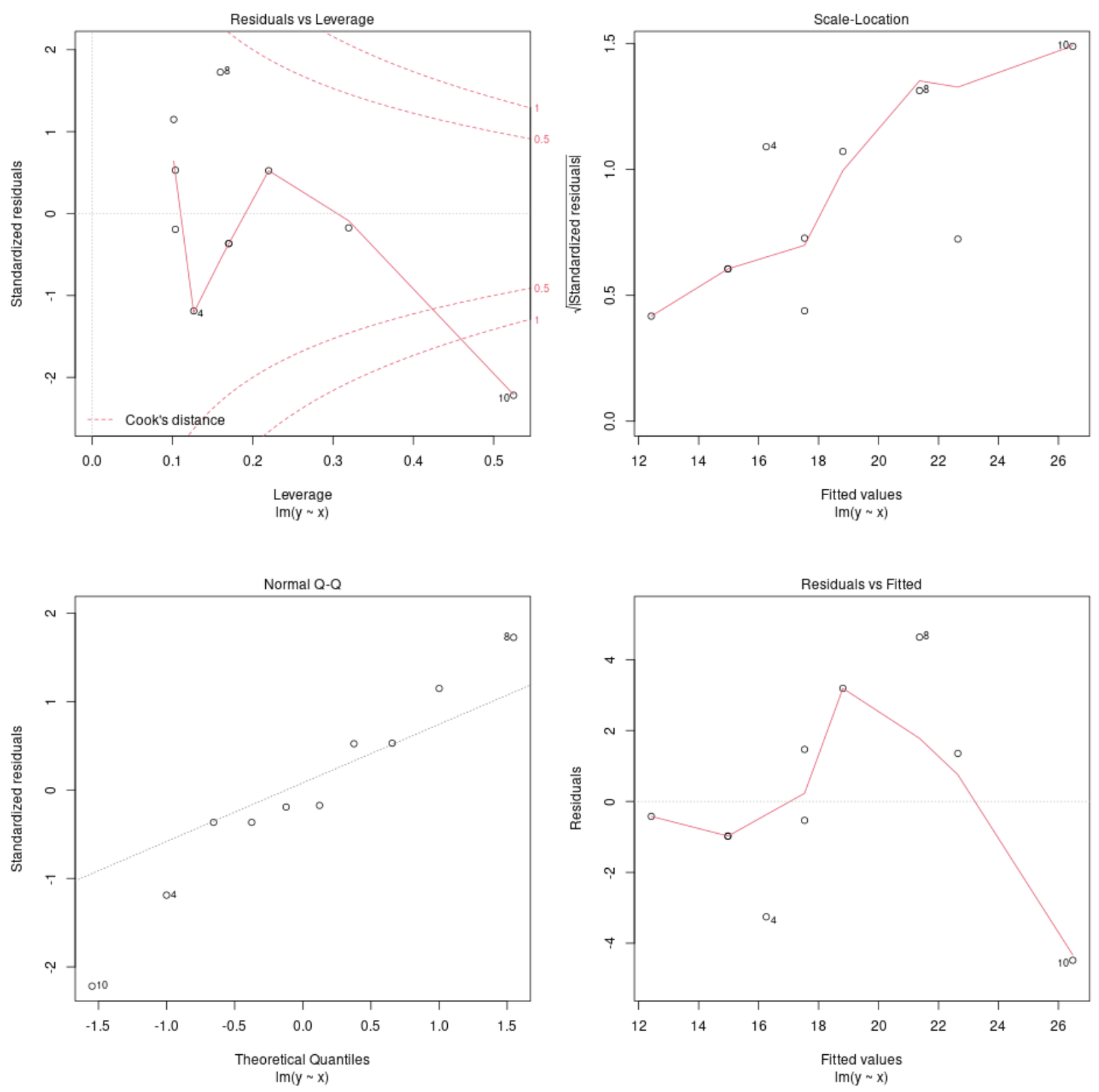
These plots allow us to analyze the residuals of the regression model to determine if the model is appropriate to use for the data.
Refer to this tutorial for a complete explanation of how to interpret the diagnostic plots for a model in R.
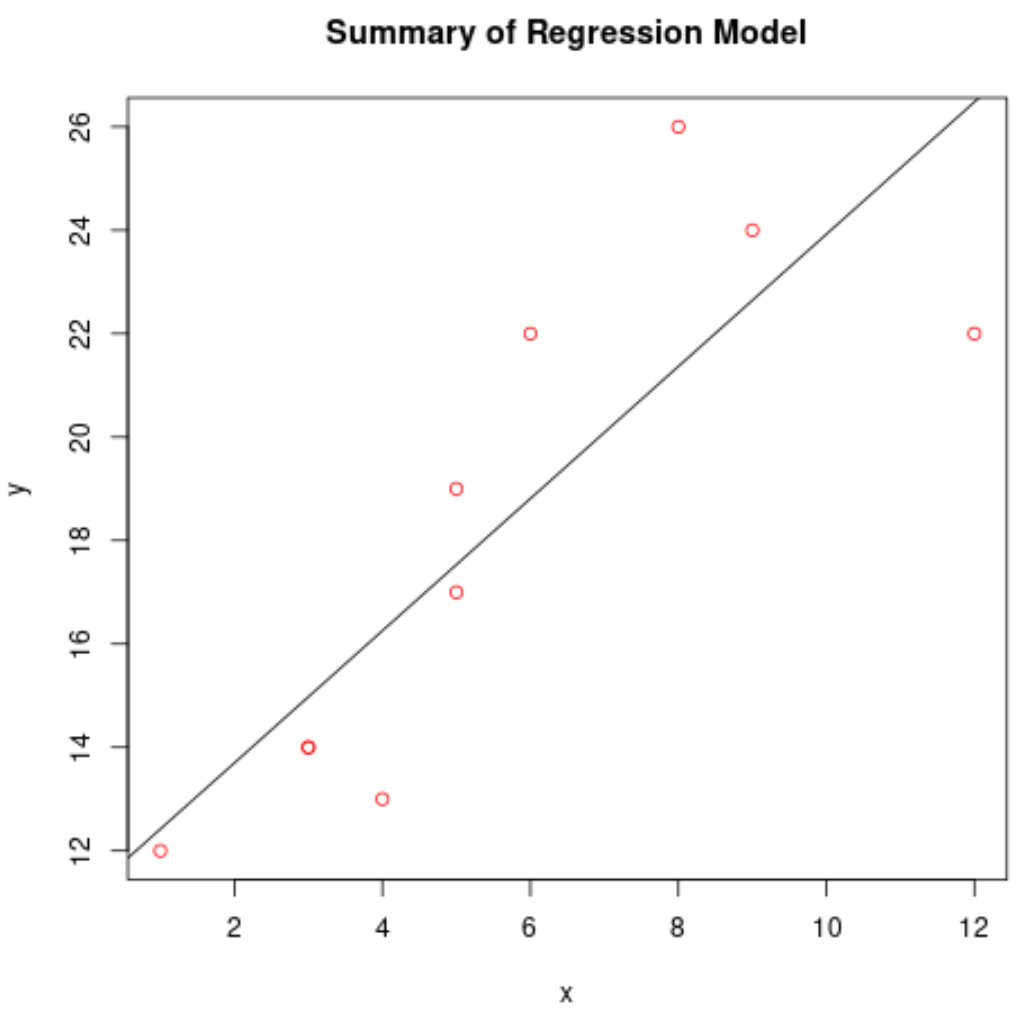
Plot the Fitted Regression Model
We can use the abline() function to plot the fitted regression model:
#create scatterplot of raw data
plot(df$x, df$y, col='red', main='Summary of Regression Model', xlab='x', ylab='y')

#add fitted regression line
abline(model)
Use the Regression Model to Make Predictions
We can use the predict() function to predict the response value for a new observation:
#define new observation
new frame(x=c(5))

#use the fitted model to predict the value for the new observation
predict(model, newdata = new)

      1
17.5332
The model predicts that this new observation will have a response value of 17.5332.
Additional Resources
How to Perform Simple Linear Regression in R
How to Perform Multiple Linear Regression in R
How to Perform Stepwise Regression in R