Levene’s Test is used to determine whether two or more groups have equal variances. This is a widely used test in statistics because many statistical tests use the assumption that groups have equal variances.
This tutorial explains how to perform Levene’s Test in Excel.
Example: Levene’s Test in Excel
Researchers want to know if three different fertilizers lead to different levels of plant growth. They randomly select 30 different plants and split them into three groups of 10, applying a different fertilizer to each group. At the end of one month they measure the height of each plant.
Before they conduct a statistical test to determine if there is a difference in plant growth between the groups, they first want to perform Levene’s Test to determine whether or not the three groups have equal variances.
Use the following steps to perform Levene’s Test in Excel.
Step 1: Enter the data.
Enter the following data, which shows the total growth (in inches) for each of the 10 plants in each group:

Step 2: Calculate the mean of each group.
Next, calculate the mean of each group using the AVERAGE() function:

Step 3: Calculate the absolute residuals.
Next, calculate the absolute residuals for each group. The following screenshot shows the formula to use to calculate the residual of the first observation in the first group:

Copy this formula to all remaining cells:

Step 4: Perform a One-Way ANOVA.
Excel doesn’t have a built-in function to perform Levene’s Test, but a workaround is to perform a one-way ANOVA on the absolute residuals. If the p-value from the ANOVA is less than some significance level (.e.g 0.05), this indicates that the three groups do not have equal variances.
To perform a one-way ANOVA, go to the Data tab and click on Data Analysis. If you don’t see this option, then you need to first install the free Analysis ToolPak.

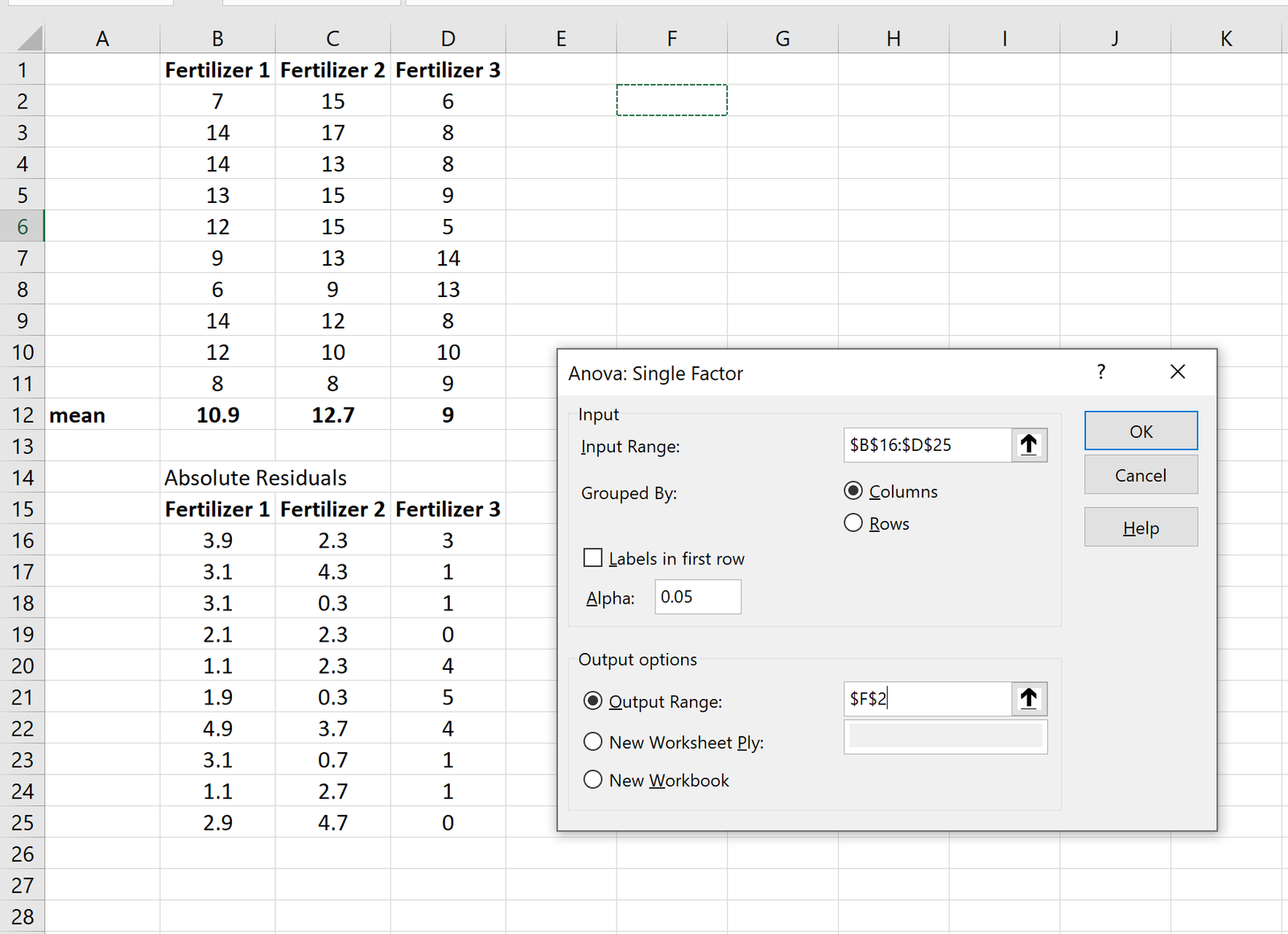
Once you click on Data Analysis, a new window will pop up. Select Anova: Single Factor and click OK.
For Input Range, choose the cells where the absolute residuals are located. For Output Range, choose a cell where you would like the results of the one-way ANOVA to appear. Then click OK.
The results of the one-way ANOVA will automatically appear:
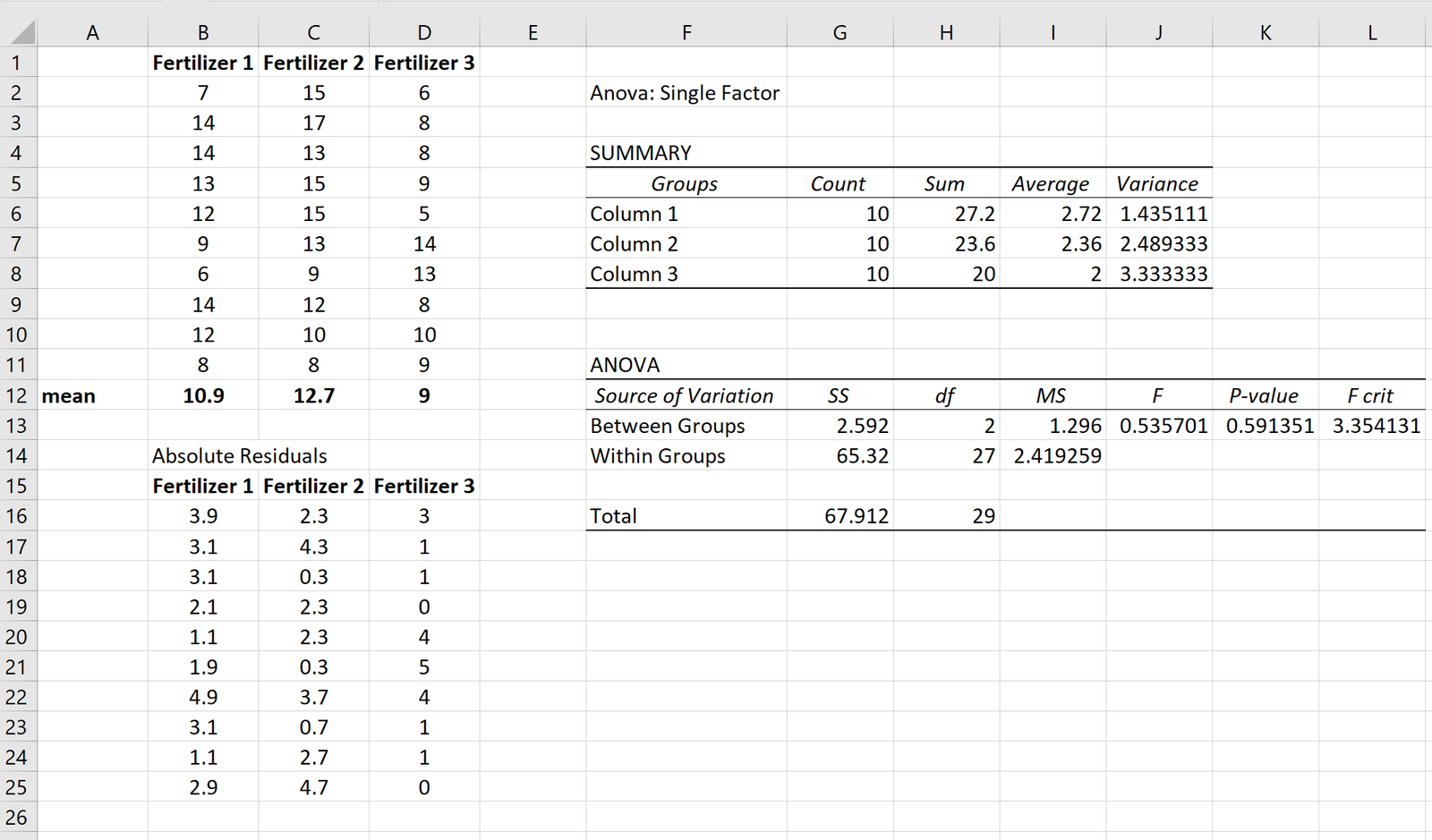
We can see that the p-value of the one-way ANOVA is 0.591251. Because this value is not less than 0.05, we fail to reject the null hypothesis. In other words, we don’t have sufficient evidence to say that the variance between the three groups is different.