How to Perform a Jarque-Bera Test in Excel

The Jarque-Bera test is a goodness-of-fit test that determines whether or not sample data have skewness and kurtosis that matches a normal distribution.

The test statistic of the Jarque-Bera test is always a positive number and if it’s far from zero, it indicates that the sample data do not have a normal distribution.

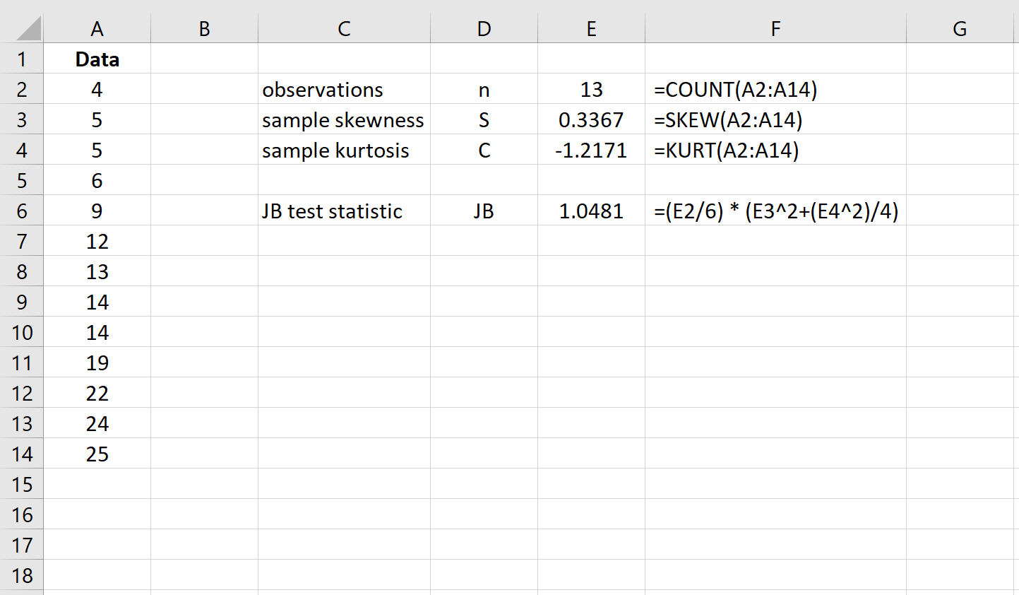
The test statistic JB is defined as:

JB  =(n/6) * (S² + (C²/4))

where:

• n: the number of observations in the sample
• S: the sample skewness
• C: the sample kurtosis

Under the null hypothesis of normality, JB ~ X²(2)

This tutorial explains how to conduct a Jarque-Bera test in Excel.

Jarque-Bera test in Excel

Use the following steps to perform a Jarque-Bera test for a given dataset in Excel.

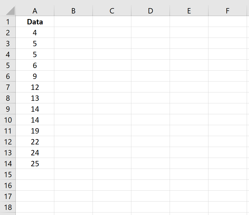
Step 1: Input the data.

First, input the dataset into one column:

Step 2: Calculate the Jarque-Bera Test Statistic.

Next, calculate the JB test statistic. Column F shows the formulas used:

Step 3: Calculate the p-value of the test.

Recall that under the null hypothesis of normality, the test statistic JB follows a Chi-Square distribution with 2 degrees of freedom. Thus, to find the p-value for the test we will use the following function in Excel: =CHISQ.DIST.RT(JB test statistic, 2)

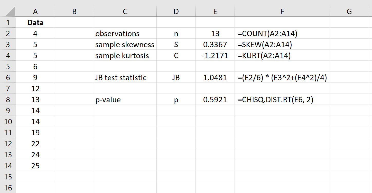
The p-value of the test is 0.5921. Since this p-value is not less than 0.05, we fail to reject the null hypothesis. We don’t have sufficient evidence to say that the dataset is not normally distributed.