You can use the following basic syntax to replace #N/A values in Google Sheets with either zeros or blanks:
#replace #N/A with zero
=IFERROR(FORMULA, "0")

#replace #N/A with blank
=IFERROR(FORMULA, "")
The following example shows how to use this syntax in practice to replace #N/A values from a VLOOKUP with zero or blanks.
Related: How to Replace Blank Cells with Zero in Google Sheets
Example: Replace #N/A Values in Google Sheets
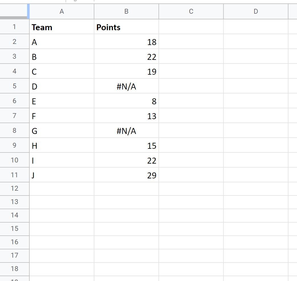
Suppose we have the following dataset in Google Sheets that shows the team name and points scored for various basketball teams:
And suppose we use the VLOOKUP() function to look up points based on team name:

Notice that some of the values returned in the VLOOKUP() are #N/A values.
We can turn these values into zeros by using the IFERROR() function as follows:
=IFERROR(VLOOKUP(A2, $A$2:$B$11, 2, FALSE), "0")
The following screenshot shows how to use this function in practice:
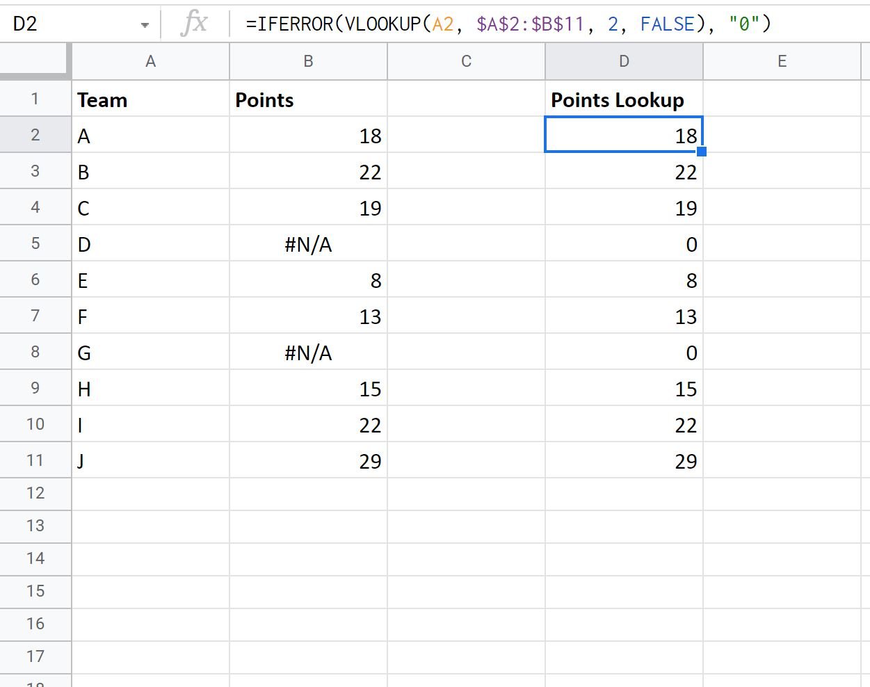
Notice that the VLOOKUP() function now returns 0 instead of #N/A values.
Alternatively, we can turn the #N/A values into blanks using the IFERROR() function as follows:
#replace #N/A with blank
=IFERROR(VLOOKUP(A2, $A$2:$B$11, 2, FALSE), "")
The following screenshot shows how to use this function in practice:
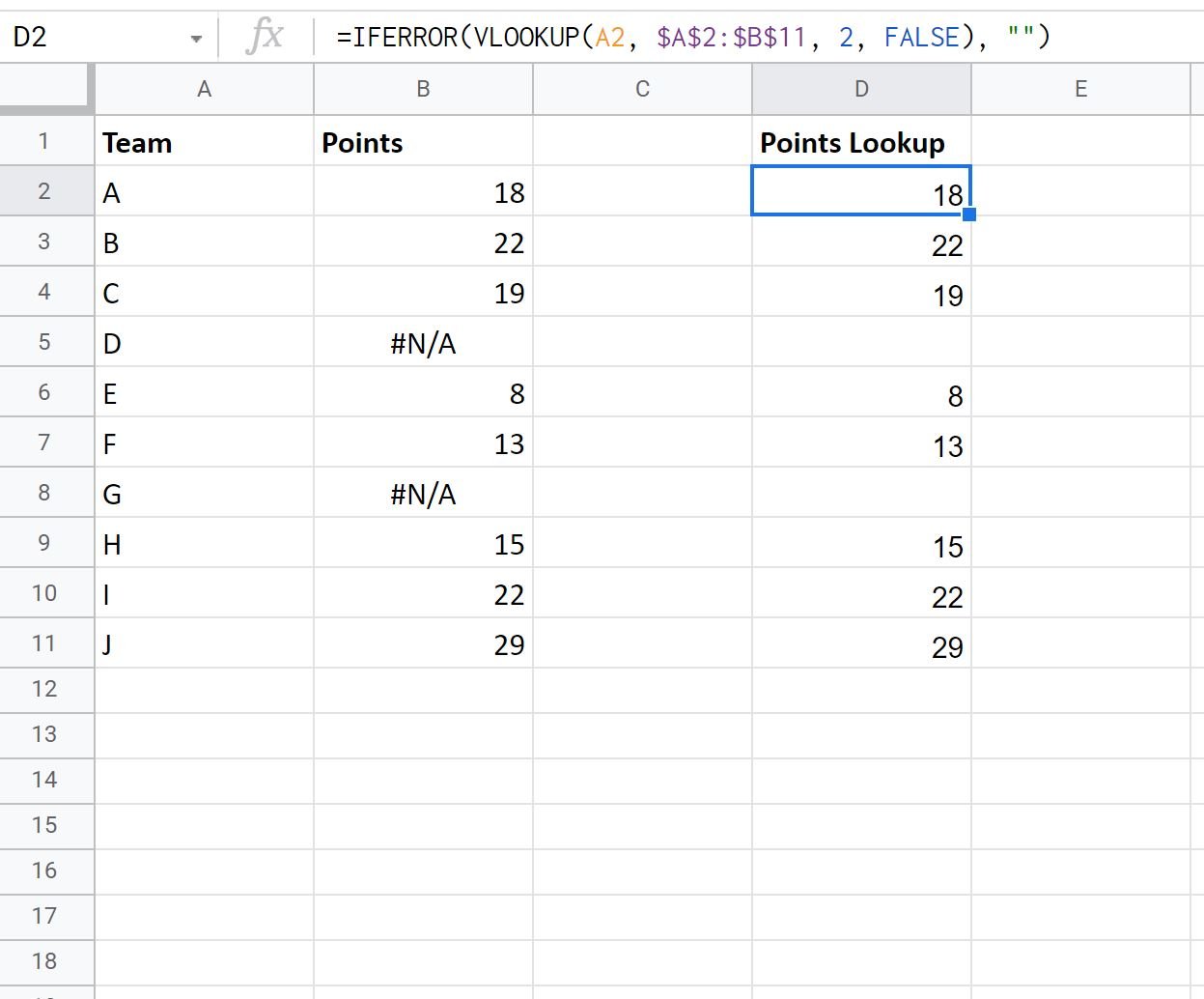
Notice that each value that was previously #N/A is now blank.
It’s worth noting that we can use the IFERROR() function to replace #N/A values with any value that we’d like.
In the previous examples we simply replaced #N/A values with zeros or blanks because these are the most common replacement values used in practice.
Additional Resources
The following tutorials explain how to perform other common tasks in Google Sheets:
How to Ignore Blank Cells with Formulas in Google Sheets
How to Ignore #N/A Values with Formulas in Google Sheets