This step-by-step tutorial explains how to create the following progress bars in Google Sheets:
Step 1: Enter the Data
First, let’s enter some data that shows the progress percentage for 10 different tasks:

Step 2: Add the Progress Bars
Next, type the following formula into cell C2 to create a progress bar for the first task:
=SPARKLINE(B2,{"charttype","bar";"max",1;"min",0;"color1","green"})
Copy and paste this formula down to every remaining cell in column C:
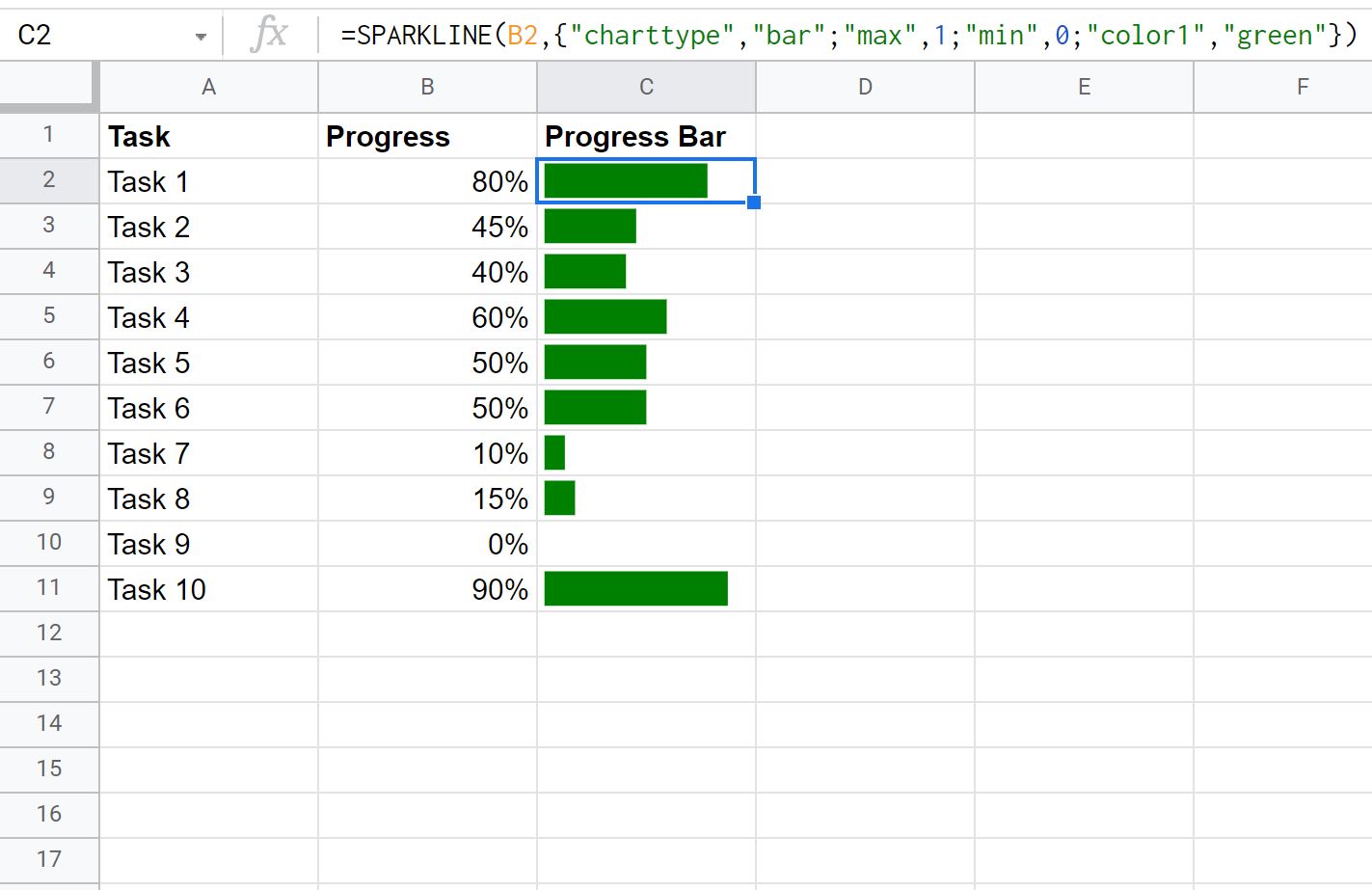
The length of each progress bar in column C reflects the percentage value in column B.
Step 3: Format the Progress Bars (Optional)
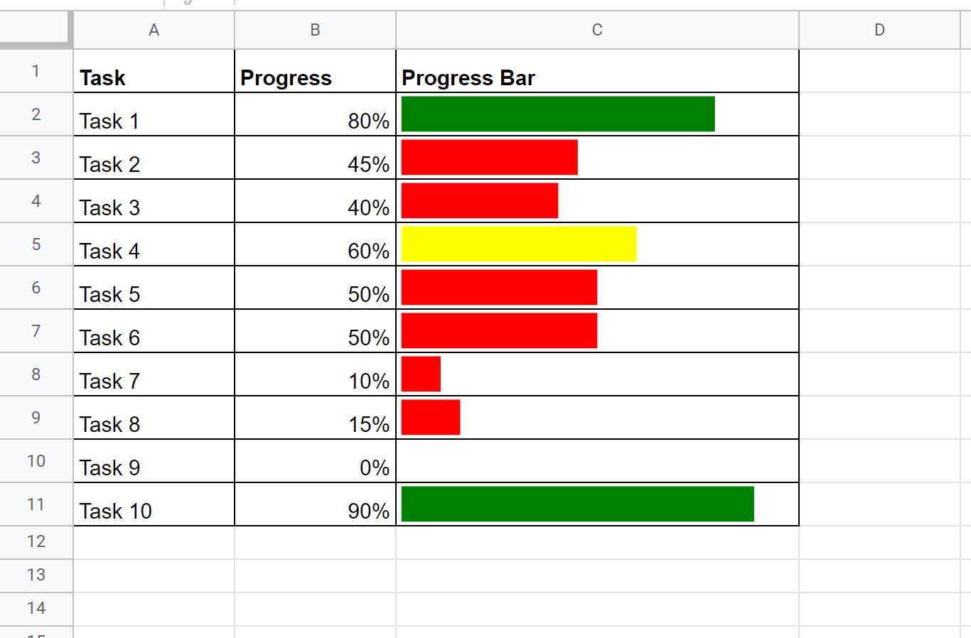
You can modify the progress bars to display specific colors based on the progress percentage.
For example, you can use the following formula to display a green progress bar if the percentage is greater than 70, else a yellow progress bar if the percentage is greater than 50, else a red progress bar:
=SPARKLINE(B2,{"charttype","bar";"max",1;"min",0;"color1",IF(B2>0.7,"green",IF(B2>0.5,"yellow","red"))})
The following screenshot shows how to use this formula in practice:

The color of the progress bar is now dependent on the value in column B.
Feel free to add a border around the cells and increase the length and width of the cells to make the progress bars larger and easier to read:
Additional Resources
The following tutorials explain how to create other common visualizations in Google Sheets:
How to Plot Multiple Lines in Google Sheets
How to Create an Area Chart in Google Sheets
How to Create a Gauge Chart in Google Sheets