You can use the following formulas to create an IF function with 3 conditions in Google Sheets:
Method 1: Nested IF Function
=IF(C215, "Bad", IF(C220, "OK", IF(C225, "Good", "Great")))
Method 2: IF Function with AND Logic
=IF(AND(A2="Mavs", B2="Guard", C2>25), "Yes", "No")
Method 3: IF Function with OR Logic
=IF(OR(A2="Mavs", B2="Guard", C2>25), "Yes", "No")
The following examples show how to use each formula in practice with the following dataset in Google Sheets:

Example 1: Nested IF Function
We can type the following formula into cell D2 to return a specific value based on the value for each player in the Points column:
=IF(C215, "Bad", IF(C220, "OK", IF(C225, "Good", "Great")))
We can then drag and fill this formula down to each remaining cell in column D:
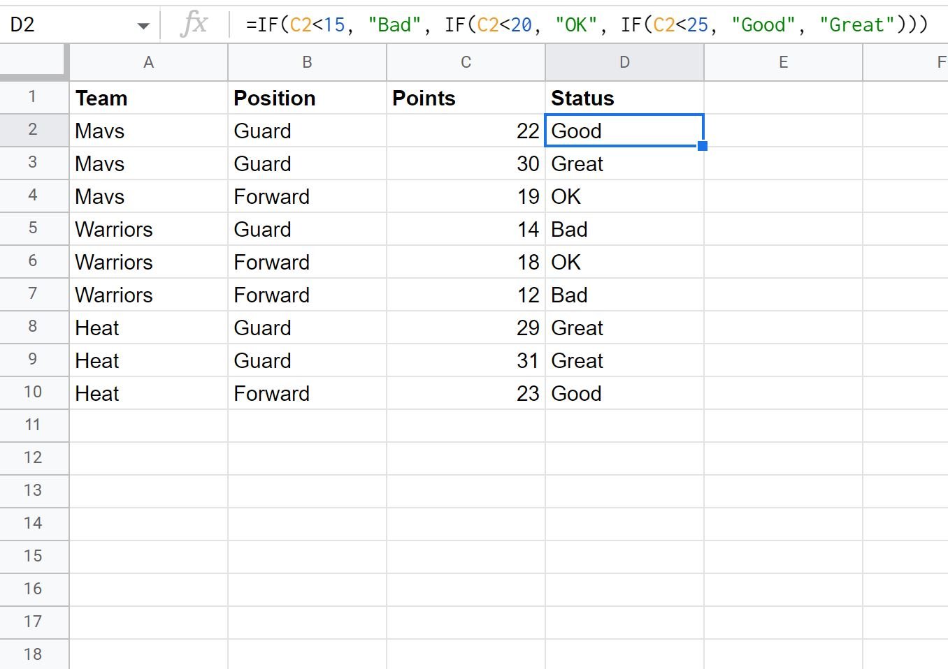
Here’s what this formula did:
- If the value in the Points column is less than 15, return Bad.
- Else, if the value in the Points column is less than 20, return OK.
- Else, if the value in the Points column is less than 25, return Good.
- Else, return Great.
Example 2: IF Function with AND Logic
We can type the following formula into cell D2 to return “Yes” if three conditions are met for a specific player or “No” if at least one of the conditions is not met:
=IF(AND(A2="Mavs", B2="Guard", C2>25), "Yes", "No")
We can then drag and fill this formula down to each remaining cell in column D:

Here’s what this formula did:
- If the value in the Team column was “Mavs” and the value in the Position column was “Guard” and the value in the Points column was greater than 25, return Yes.
- Else, if at least one condition is not met then return No.
Notice that only one row returned “Yes” because only one row met all three conditions.
Example 3: IF Function with OR Logic
We can type the following formula into cell D2 to return “Yes” if one of three conditions are met for a specific player or “No” if none of the conditions are met:
=IF(OR(A2="Mavs", B2="Guard", C2>25), "Yes", "No")
We can then drag and fill this formula down to each remaining cell in column D:

Here’s what this formula did:
- If the value in the Team column was “Mavs” or the value in the Position column was “Guard” or the value in the Points column was greater than 25, return Yes.
- Else, if none of the conditions are met then return No.
Notice that six total rows returned “Yes” because each of those rows met at least one of the three conditions.
Additional Resources
The following tutorials explain how to perform other common tasks in Google Sheets:
Google Sheets: How to COUNTIF Not Equal to Text
Google Sheets: Calculate Average if Greater Than Zero
Google Sheets: How to Calculate Average If Cell Contains Text