Often you may want to group data by week in Google Sheets.
Fortunately this is easy to do using the WEEKNUM() function.
The following step-by-step example shows how to use this function to group data by week in Google Sheets.
Related: How to Group Data by Month in Google Sheets
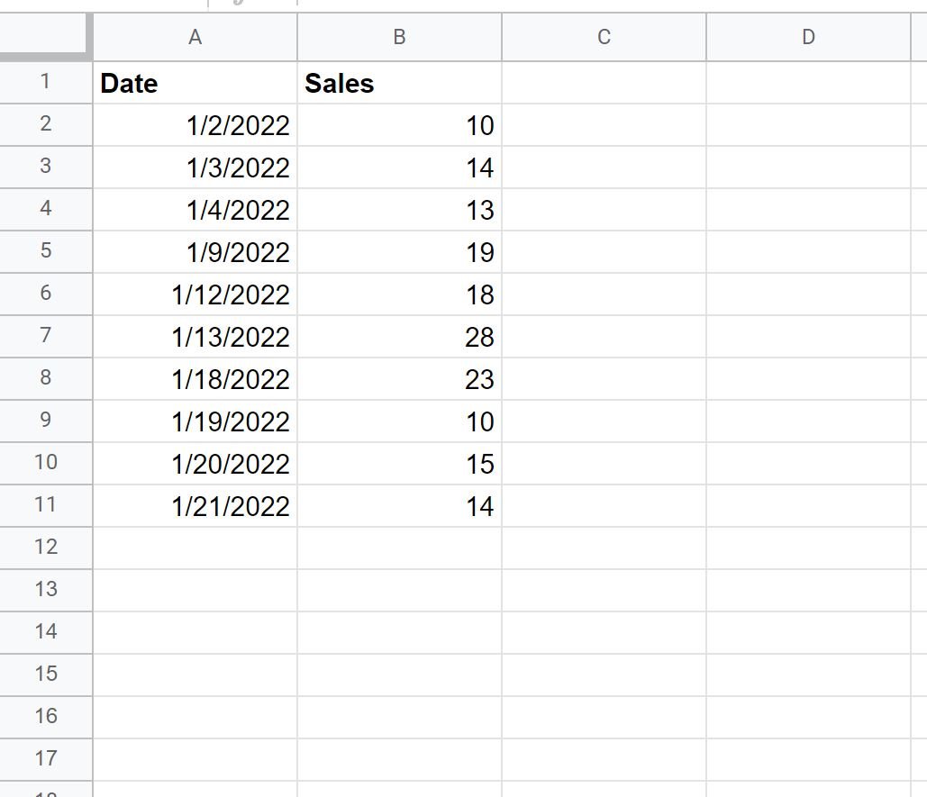
Step 1: Create the Data
First, let’s create a dataset that shows the total sales made by some company on various days:
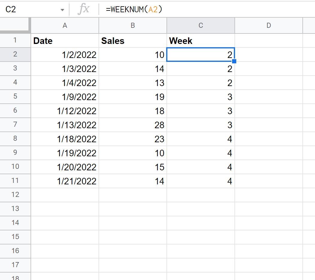
Step 2: Create Week Variable
To extract the week of the year from the Date column, we can use the WEEKNUM() function to return a value between 1 and 53.
We can type in the following formula in cell C2:
=WEEKNUM(A2)
We can then copy and paste this formula down to the remaining cells in column C:
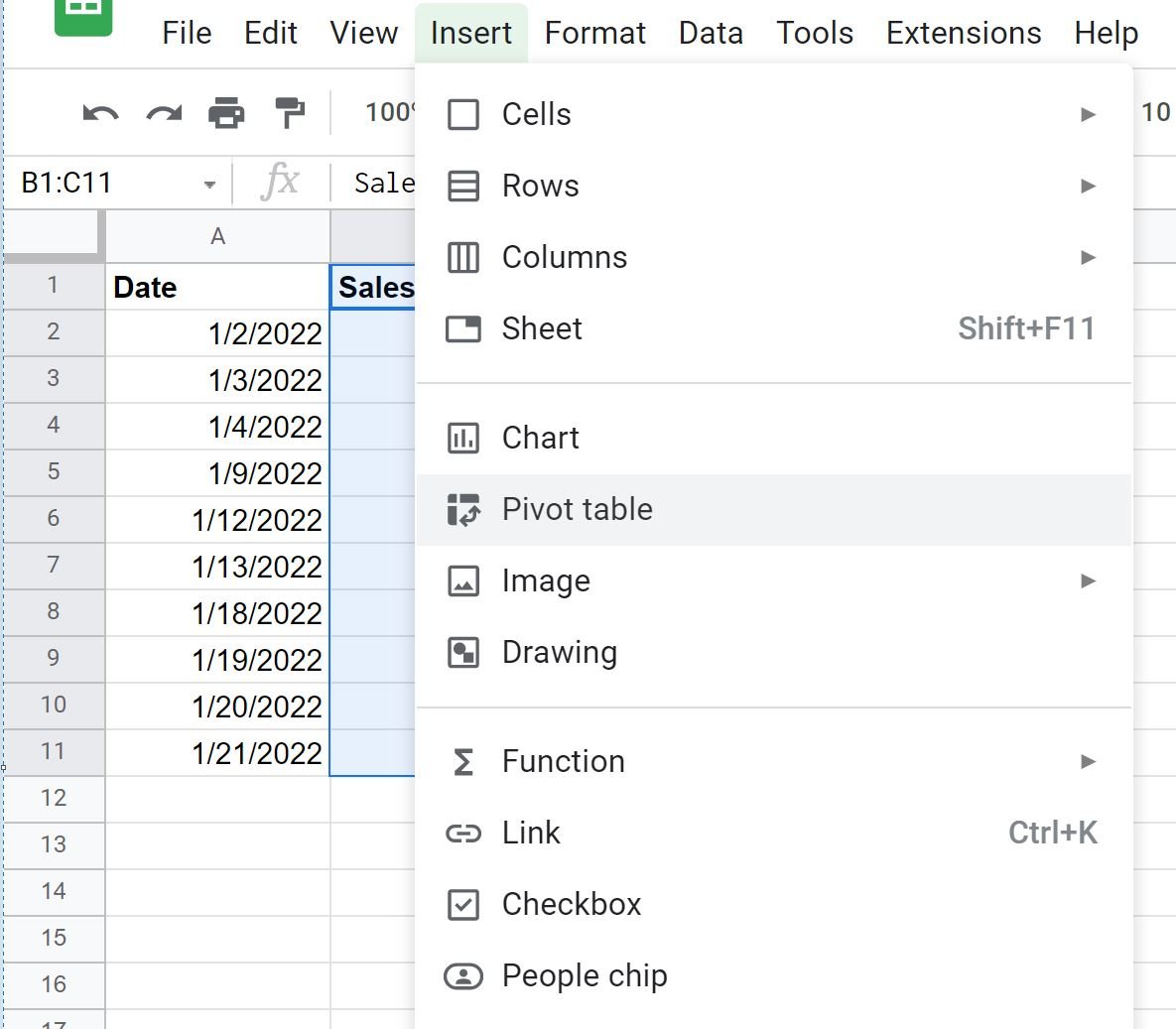
Step 3: Create a Pivot Table
Lastly, we can create a pivot table to find the sum of sales made each week.
To create a pivot table, highlight the cells in the range B1:C11 and then click the Insert tab along the top ribbon and click Pivot table.
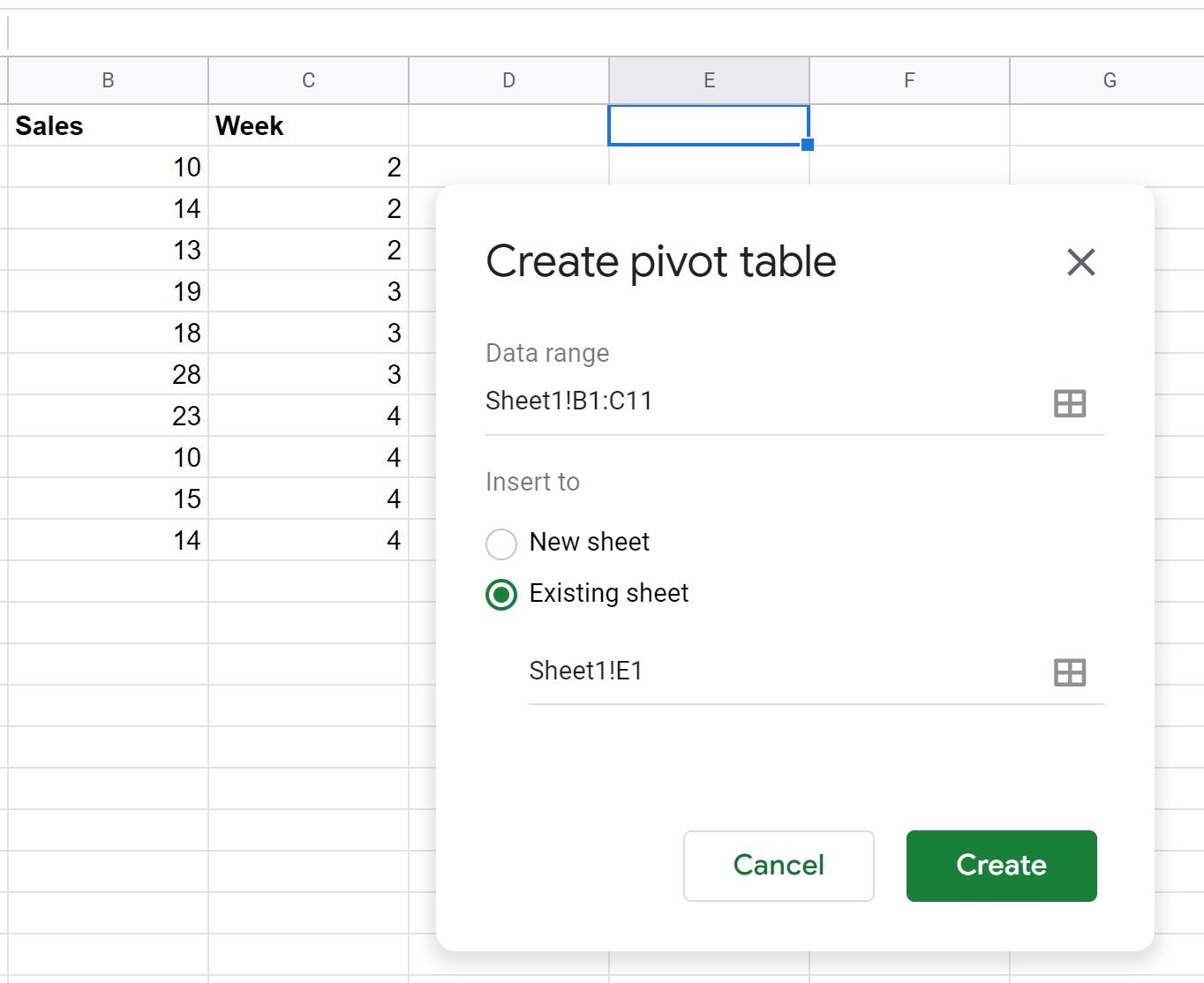
Next, we’ll choose to insert the pivot table in the current worksheet in cell E1 and click Create:
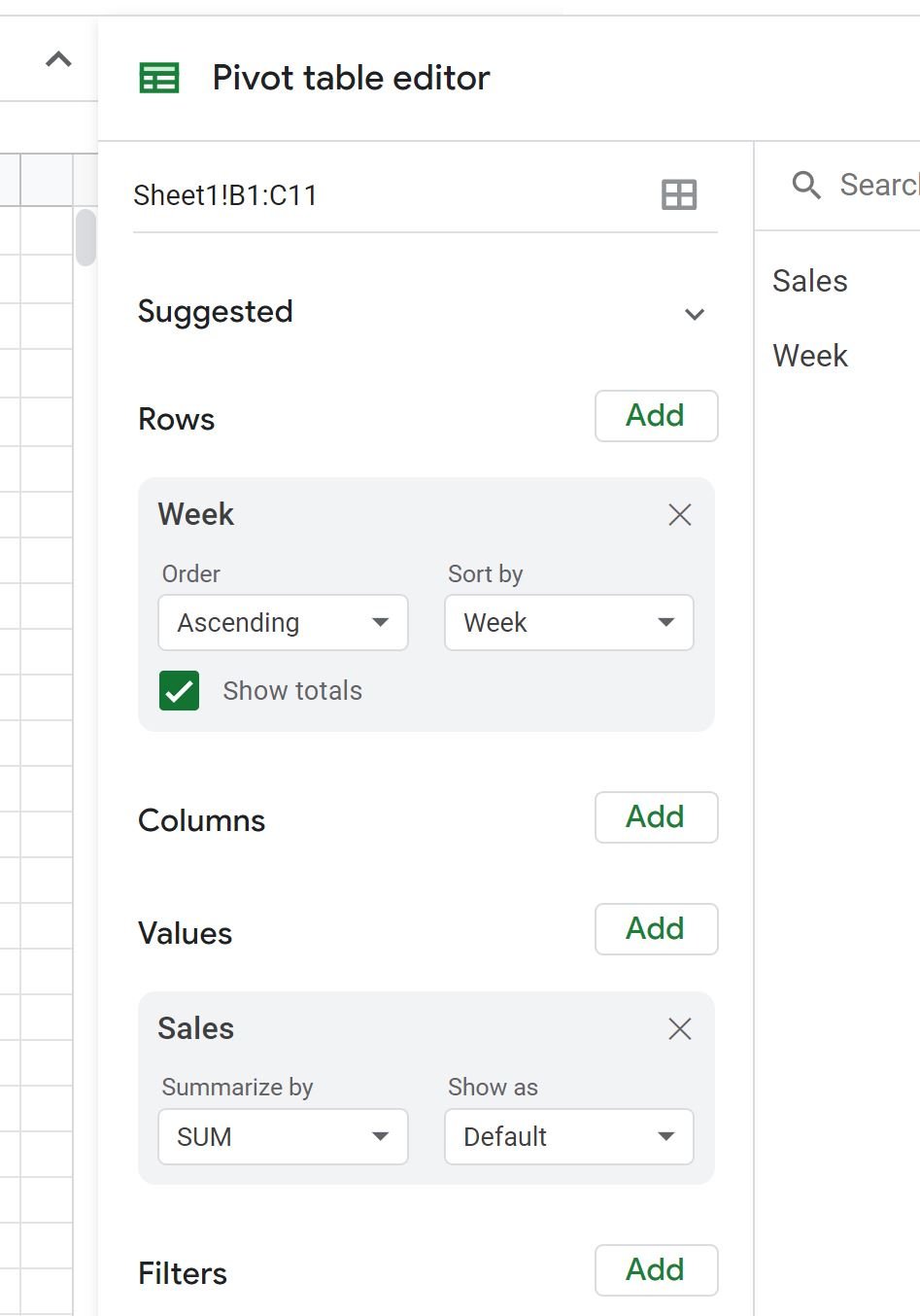
In the Pivot table editor on the right side of the screen, choose Week for the Rows and Sales for the Values:
The values in the pivot table will now be filled in.
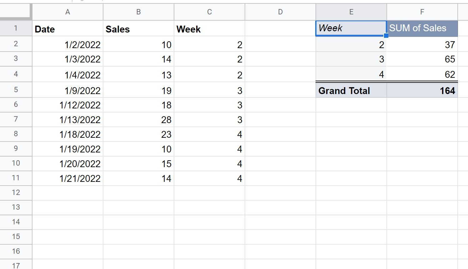
From the pivot table we can see:
- The total sales made during week 2 were 37.
- The total sales made during week 3 were 65.
- The total sales made during week 4 were 62.
We can also see that the grand total of sales made was 164.
Additional Resources
The following tutorials explain how to perform other common operations in Google Sheets:
Google Sheets: How to Filter for Cells that Contain Text
Google Sheets: How to Use SUMIF with Multiple Columns
Google Sheets: How to Sum Across Multiple Sheets