Often you may want to find duplicate values across two columns in Google Sheets.
Fortunately this is easy to do using conditional formatting along with the COUNTIF() function.
The following example shows how to find duplicate values across two columns in the following dataset in Google Sheets:

Let’s jump in!
Example: Find Duplicates in Two Columns in Google Sheets
Suppose we have the following two columns in Google Sheets that contain the names of basketball players on two teams:

Now suppose that we would like to highlight the duplicate names across both columns.
To do so, we can highlight the cells in the range A2:B9, then click the Format tab, then click Conditional formatting:

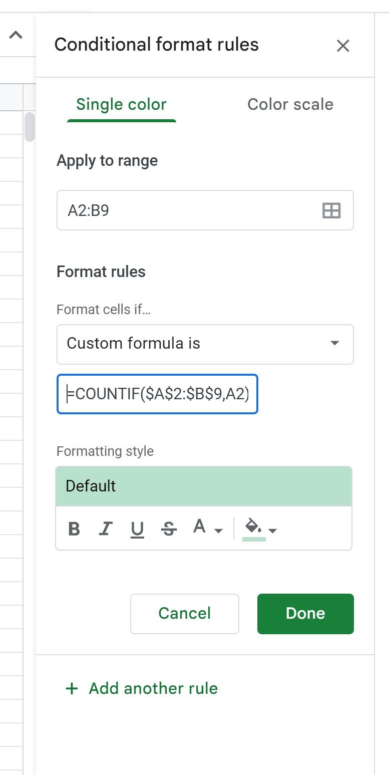
In the Conditional format rules panel that appears, click the dropdown menu under Format cells if and choose Custom formula is, then type the following formula:
=COUNTIF($A$2:$B$9,A2)>1

Once you click Done, the duplicate values that occur in both columns will be highlighted in green:

We can see that the following names are duplicates across the two columns:
- Andy
- Chad
- Frank
Each of these names occur in both columns.
Note that by default, Google Sheets uses a light green background for conditional formatting.
However, you can change the background color, font color, and font style of the conditional formatting to format the duplicate values however you’d like.
Additional Resources
The following tutorials explain how to perform other common tasks in Google Sheets:
How to Use COUNTIF Contains in Google Sheets
How to Use COUNTIF with Wildcards in Google Sheets
How to Count Cells with Text in Google Sheets