You can use the custom formula function in Google Sheets to add a strikethrough to specific cells when a checkbox is checked.
The following example shows how to use the custom formula function in practice.
Example: Conditional Formatting Based on Checkbox
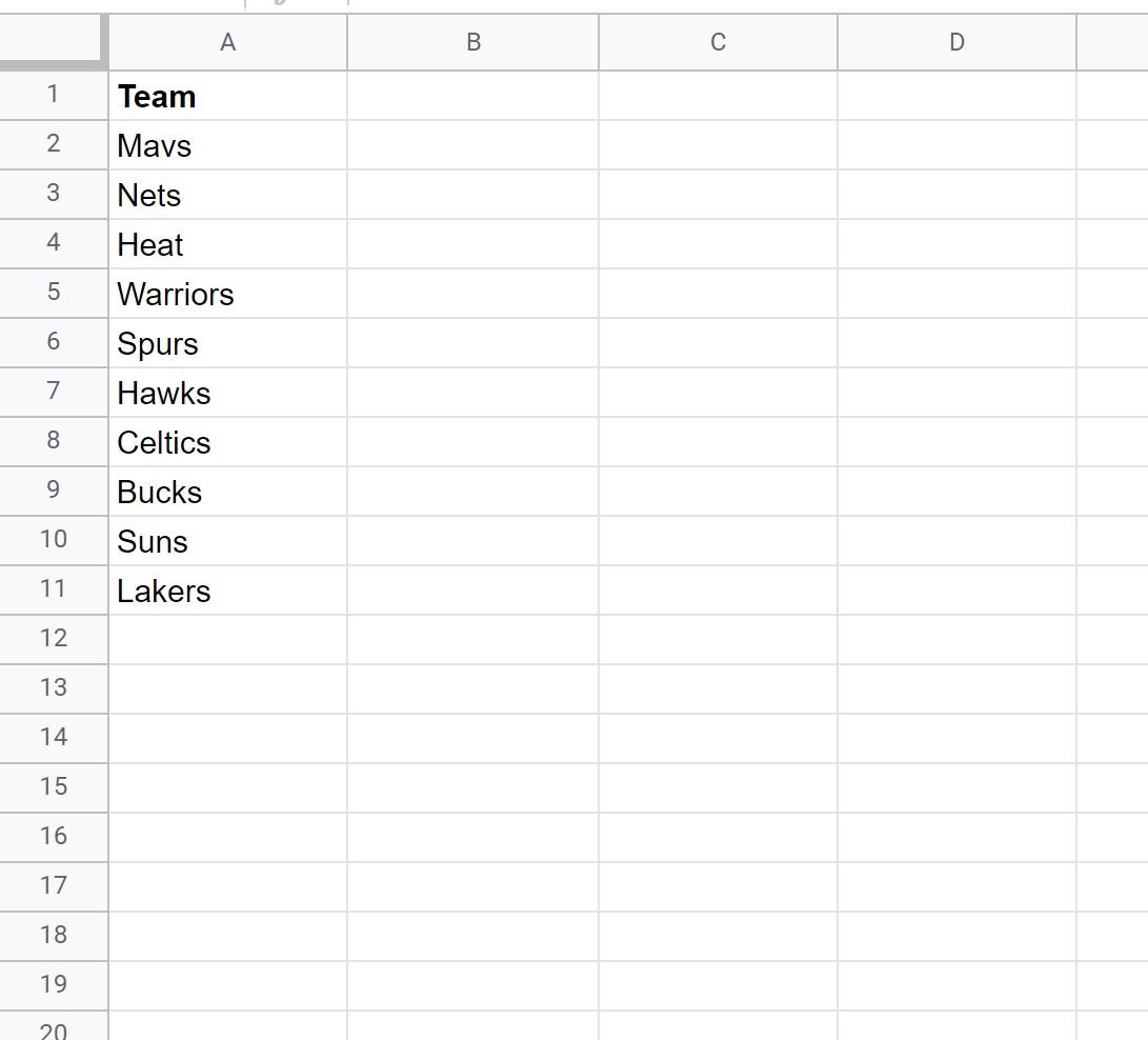
Suppose we have the following list of basketball team names in Google Sheets:
Now suppose we know that the following teams have been eliminated from the playoffs:
- Mavs
- Warriors
- Hawks
- Suns
Suppose we’d like to create a checkbox that, when checked, each of the teams that have been eliminated will have a strikethrough applied to their team name.
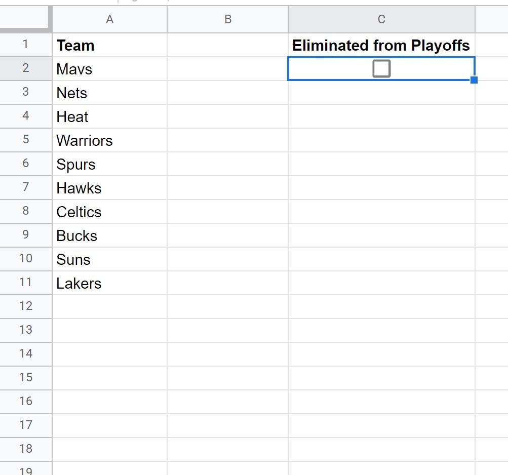
To do so, we need to first insert a checkbox by selecting cell C2, then clicking the Insert tab, then clicking Checkbox.
The following checkbox will appear:
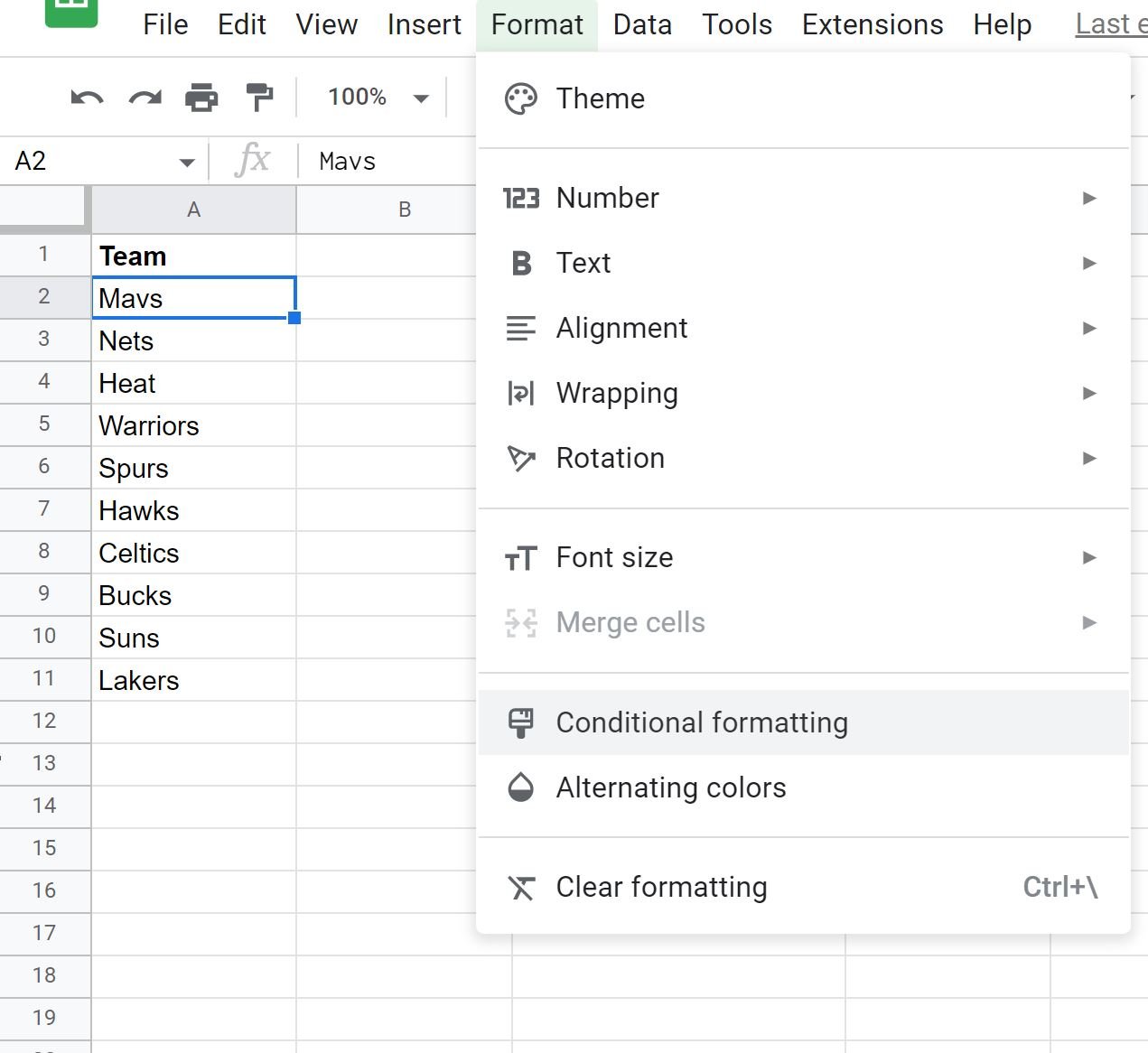
Next, click cell A2, then click the Format tab, then click Conditional formatting:
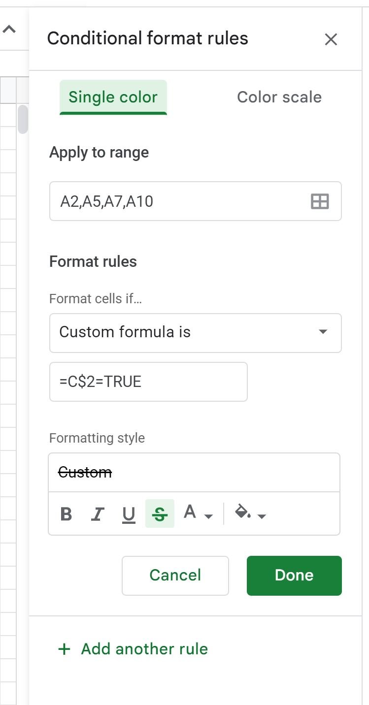
In the Conditional format rules panel that appears on the right side of the screen, type the following cells in the box called Apply to range:
A2,A5,A7,A10
Then click the Format cells if dropdown, then choose Custom formula is, then type in the following formula:
=C$2=TRUE
Note: It’s important that you include the equal sign (=) at the beginning of the formula, otherwise the conditional formatting won’t work.
Then, in the Formatting style box, click the icon that has a strikethrough symbol (to the right of the underline symbol).
Lastly, click Done.
Now when you check the checkbox in cell C2, a strikethrough will be applied to each team that has been eliminated from the playoffs:
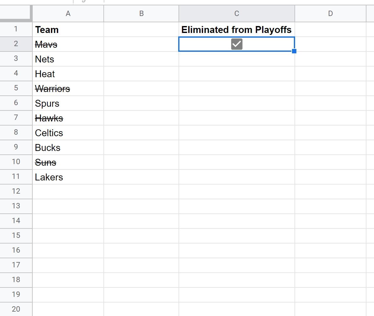
Each of the teams that have been eliminated from the playoffs now have a strikethrough applied to their team name.
Additional Resources
The following tutorials explain how to perform other common tasks in Google Sheets:
Google Sheets: How to Sum If Checkbox is Checked
Google Sheets: Conditional Formatting with Multiple Conditions
Google Sheets: Conditional Formatting if Another Cell Contains Text