You can use the following formula to calculate the average in Google Sheets only for the cells that contain a specific text:
=AVERAGEIF(A2:A13,"*text*",B2:B13)
This particular formula will calculate the average of the values in the range B2:B13 only for the cells that contain “text” in the range A2:A13.
Note: The asterisks are wildcard characters that tell Google Sheets to ignore any text before or after a specific string.
The following example shows how to use this formula in practice.
Example: Calculate Average If Cell Contains Text
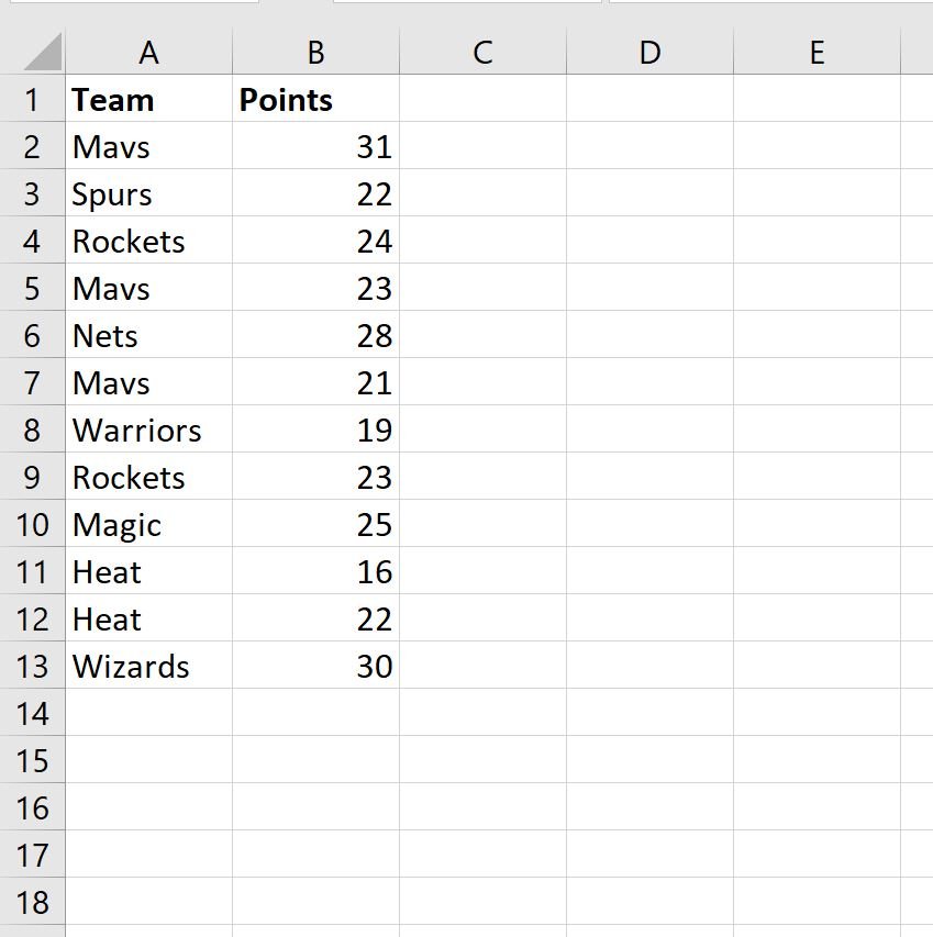
Suppose we have the following dataset that shows the points scored by 12 different basketball players:

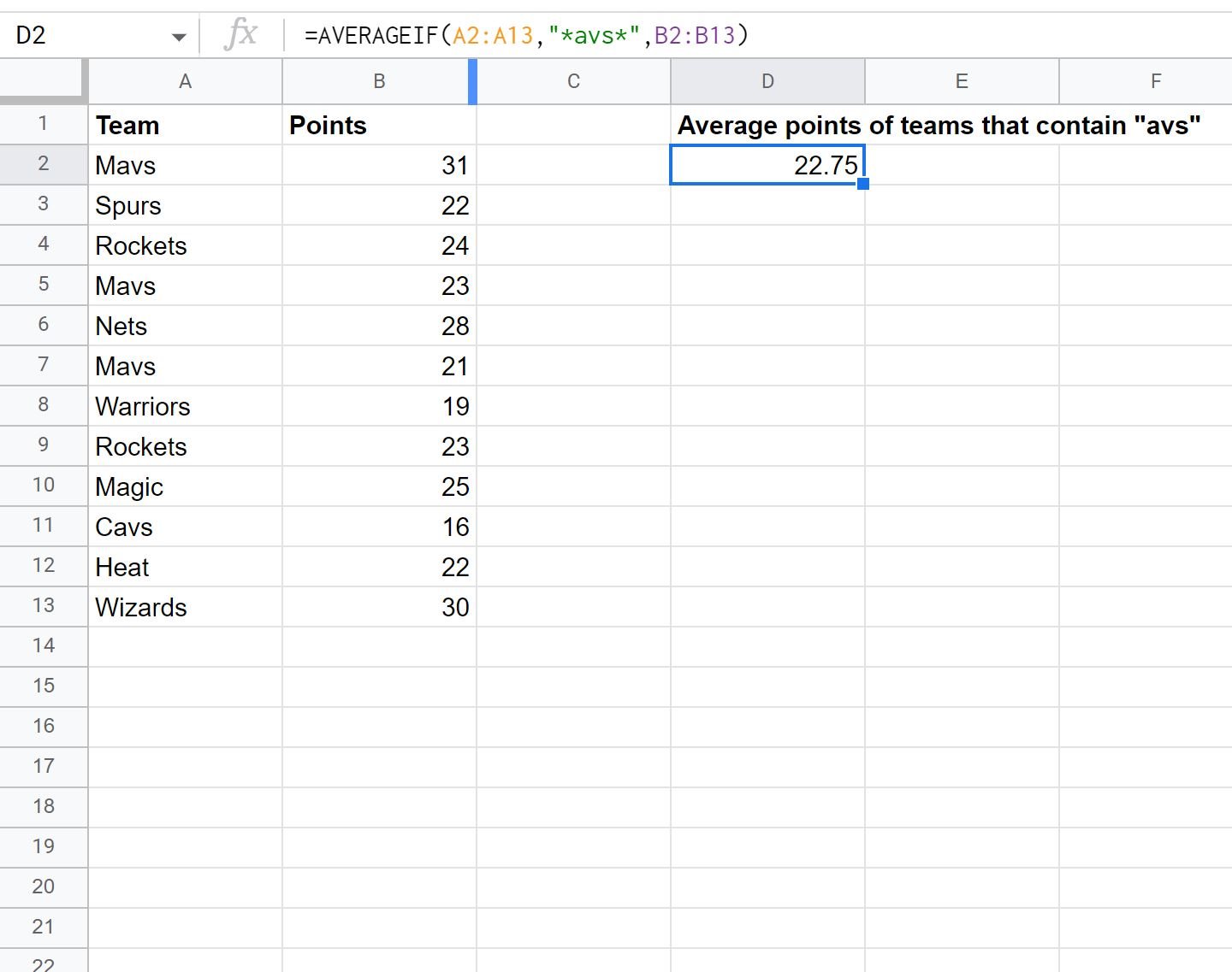
We can use the following formula to calculate the average points scored by players on any team with “avs” in the team name:
=AVERAGEIF(A2:A13,"*avs*",B2:B13)
The following screenshot shows how to use this formula in practice:

The average points scored by players on a team with “avs” in the name is 22.75.
In this particular example, there are two team names with “avs” in the name: Mavs and Cavs.
We can manually calculated the average points scored by players on these teams:
Average Points Scored = (31 + 23 + 21 +16) / 4= 22.75.
This matches the value calculated by our formula.
Note: You can find the complete documentation for the AVERAGEIF function in Google Sheets here.
Additional Resources
The following tutorials explain how to perform other common tasks in Google Sheets:
How to Use AVERAGEIFS in Google Sheets
How to Calculate Average If Not Blank in Google Sheets
How to Average Filtered Rows in Google Sheets